Analyzing Magnetic Fields in Ansys Maxwell
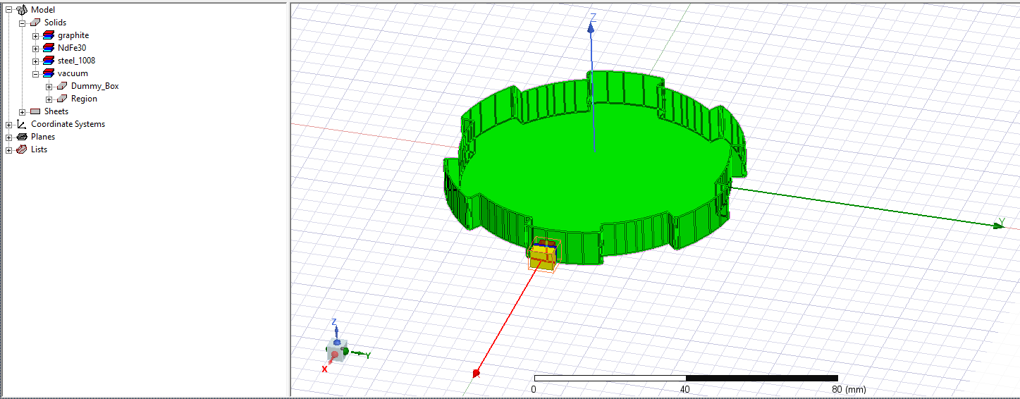
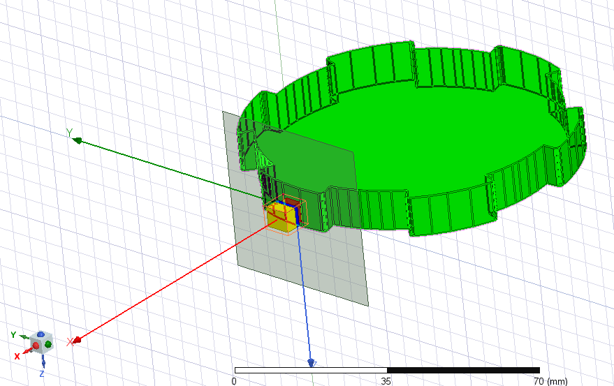
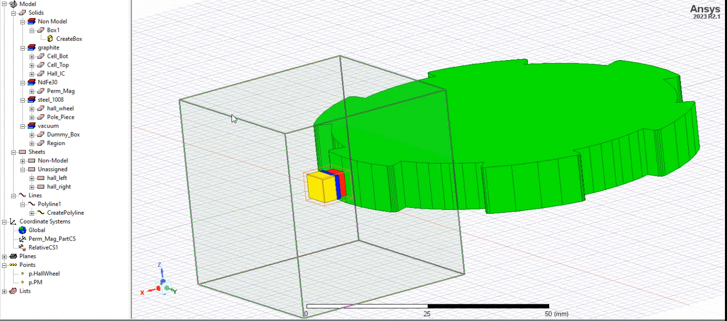
The ability to analyze magnetic fields plays a crucial role in understanding electromagnetic systems. Ansys Maxwell equips engineers with powerful tools to explore and extract valuable insights from magnetic field data. In this guide, I will delve into a few basic techniques and methods within Ansys Maxwell to analyze magnetic fields effectively.The model used for this demonstration is the Hall Sensor, found in Examples ->Maxwell -> Sensors
Section 1: Plotting Magnetic Flux Density on points, lines, surfaces, and in volumes.
Ansys Maxwell has the ability to give you magnetic field information on a wide variety of geometries. This can include individual points, objects that are part of the model, lines or planes that cut through a model, and more. This section will cover a few of the more commonly used methods.
Non-Model Objects (Non-Model Regions)
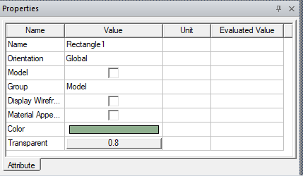
Non-model objects are a powerful feature in Ansys Maxwell. You can create them before or after solving your model. These objects help you define regions of interest for post-processing, allowing you to extract specific information without altering your initial simulation setup. This will include points, lines, planes, or 3D objects. To make an object non-model, uncheck the following box when you create the geometry.
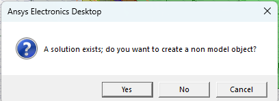
You can create non-model objects even after the simulation has been completed, you will see the following dialogue box when you try to create the geometry:
Creating Data Tables for Specific Points
Creating data tables helps you enumerate the B-field magnitude at specific points. Here's how you can achieve this:
-Create a specific point at your desired location.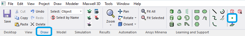
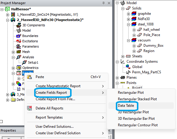
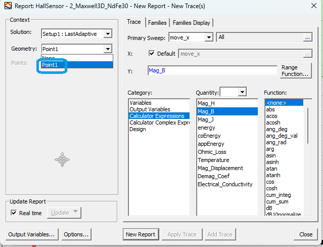
-Click On ‘New Report’ to see the results.
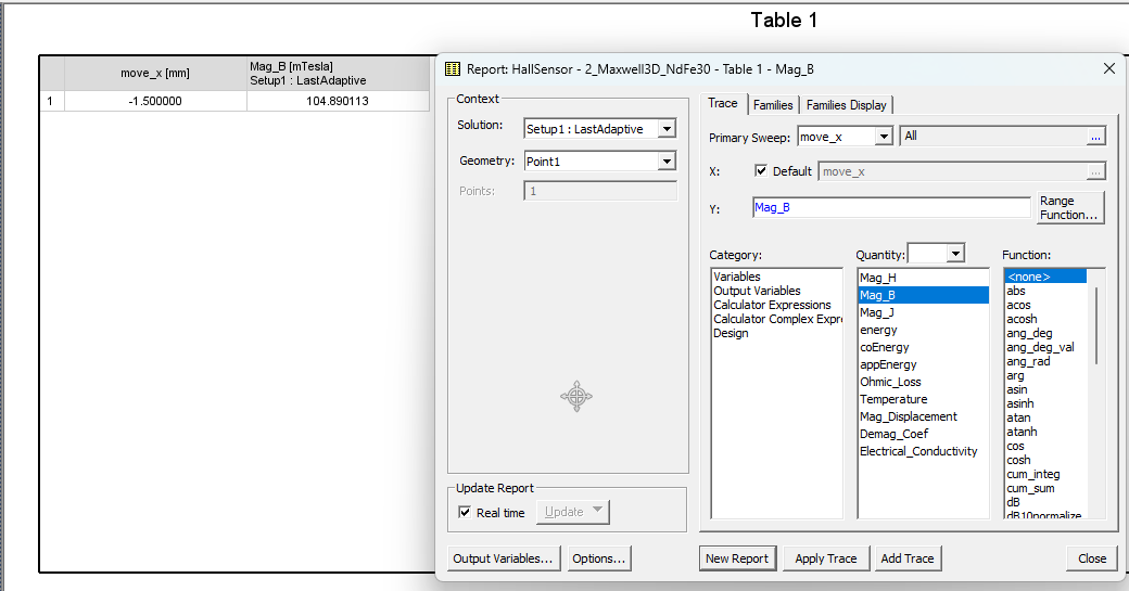
Note:
- Maxwell might prompt you to sweep a parameter when creating data tables. This may result in the first column appearing unconventional. If you find this confusing, consider the following alternative method for straightforward results.
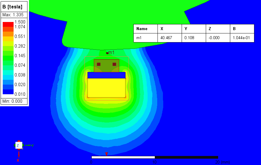
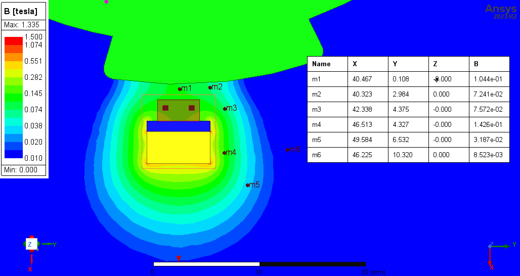
Utilizing Field Markers
Field Markers in Ansys Maxwell offer versatility. They allow you to instantly view field values at any location by simply clicking. Field Markers provide a convenient way to measure the flux density amplitude. The Markers can be created once a field plot has been created,
Simply right click on ‘Field Overlays’ and navigate to Fields->Marker->Add Marker
Click on a point you wish to place your field marker.
A table will appear that gives each marker’s name, location, and measured quantity.
Using Rectangular Plots for Line Segments
One way to visualize flux density amplitude is by drawing a line at your desired location between the magnet and the wheel within your simulation. Follow these steps:
- Open your Ansys Maxwell project.
- Select the ‘Draw’ Ribbon
- Select the ‘Draw Line’ icon
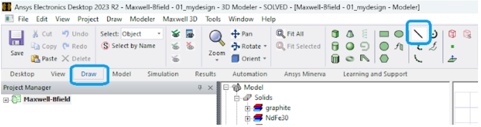
- If a solution exists, select ‘Yes’ in the dialogue box asking to create a non-model object.
- Select the two points for your line, right click, and select ‘Done’.
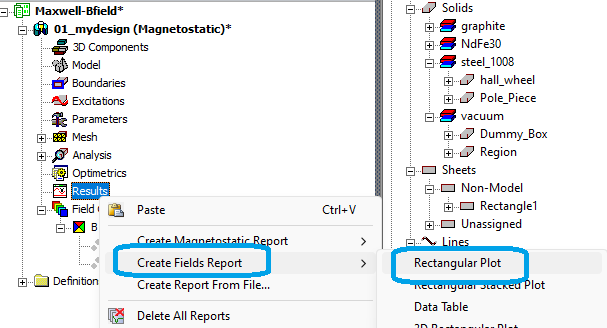
- In the model tree, select the line you created. Now right click on Results, and select ‘Create Fields Report’, and select ‘Rectangular Plot’
- In the ‘Geometry’ drop down, select the line you created.
- Select ‘Mag_B’ in the ‘Quantity’ category
- Select ‘New Report’ to see the result
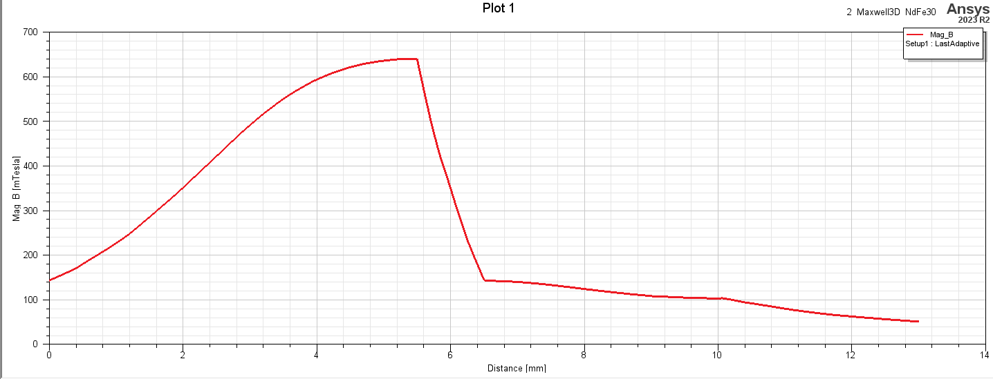
Note:
-The abscissa will always start at 0 and end at a value that represents the length of the line you have drawn.
-Version 2023R2 can not plot over a spline. To do this, try version 2022R2 or earlier.
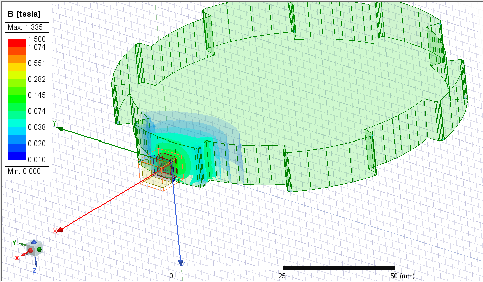
Plotting a field on a surface
One of the most common ways to visualize our magnetic field is to plot the field as a color map on a surface. This can be done for both model and non-model objects.
- Start by creating a non-model rectangle.
- With the rectangle selected, Right click on ‘Field Overlays’ and navigate to Fields->B->Mag_B
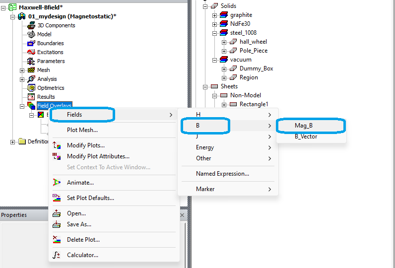
- In the box that appears, verify that Mag_B is selected under the ‘Quantity’ category, and press ‘Done’
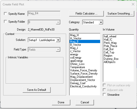
The B-field will be plotted on the rectangle you have created.
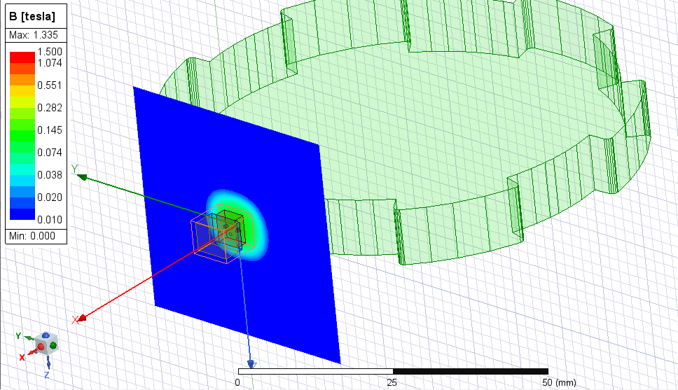
You can repeat the above steps with any other geometry. For example, this is the B-field plotted on the surface of the hall_wheel object:
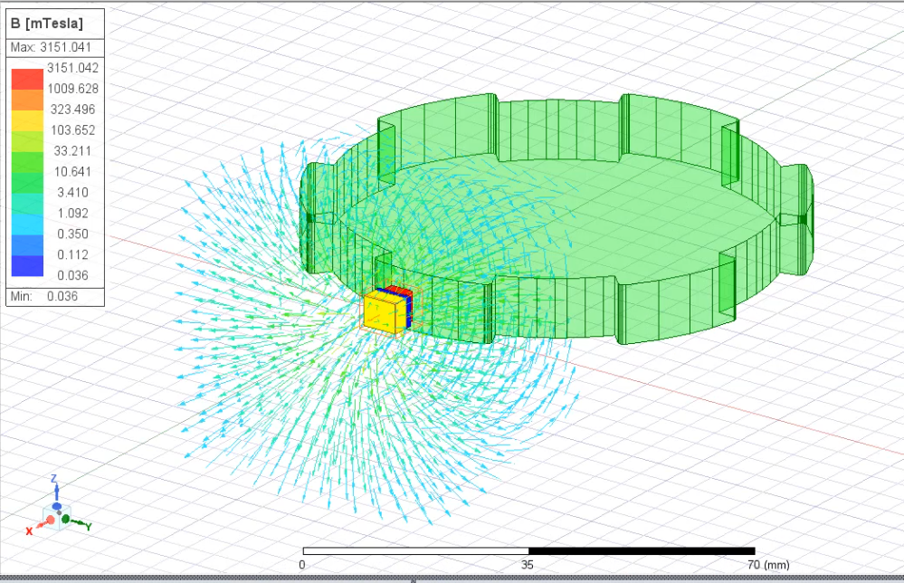
Plotting in a volume
You can create 3D objects and plot the fields inside of them.
Start by creating a non-model cube around your area of interest
Just like before, with the box selected, Right click on ‘Field Overlays’ and navigate to Fields->B
This time, select B_Vector:
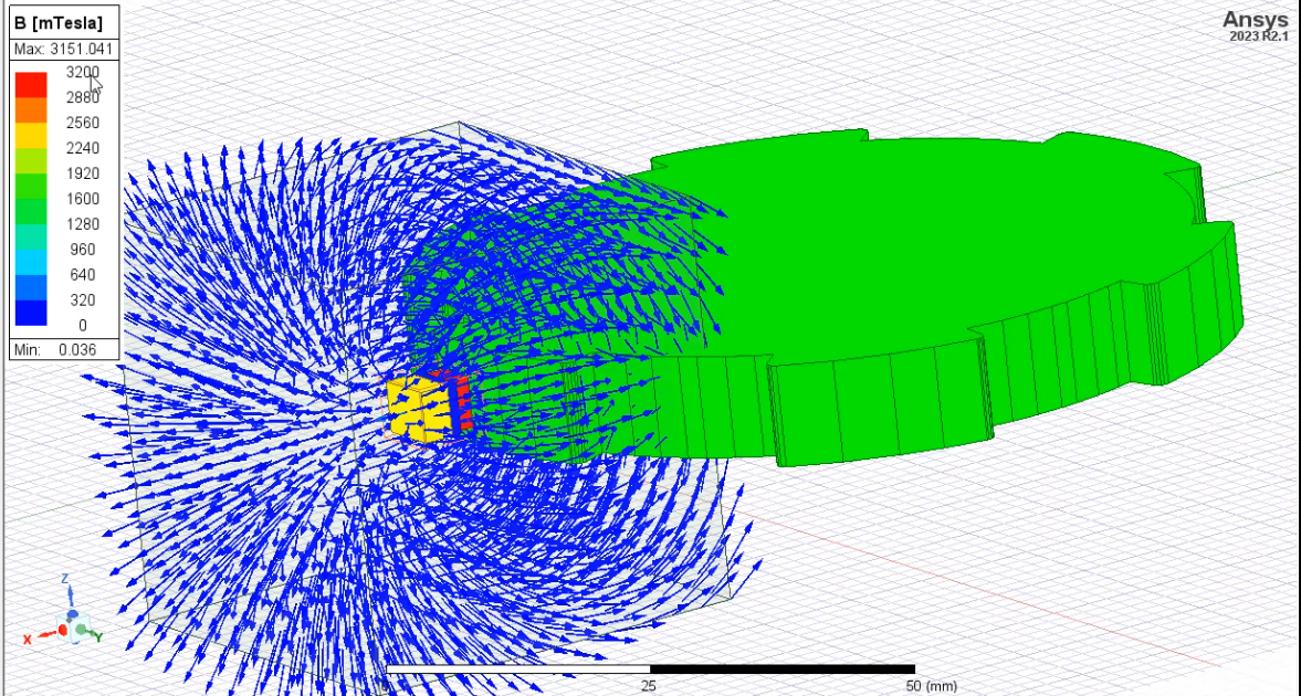
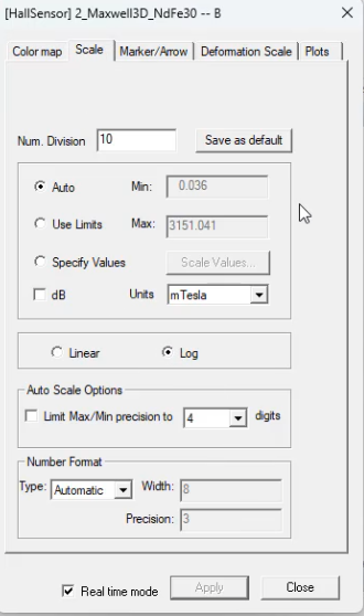
Double click on the color-key to bring up settings you can use to change the scale, spacing, size, etc., of the vectors.
Section 2: Utilizing the Fields Calculator
Sometimes, you may need to add B-field components (x, y, z) to your data tables. This additional information can enhance your analysis and provide deeper insights into magnetic fields. Ansys Maxwell offers a powerful tool for achieving this: the Fields Calculator.
The Fields Calculator in Ansys Maxwell is a versatile tool that allows you to perform various computations related to field quantities. To open the fields calculator:
- Click on Maxwell3D or Maxwell2D and select Fields->Calculator.
- Alternatively, right-click on Field Overlays in the project tree and select Calculator from the shortcut menu. This action will open the Fields Calculator dialog box.
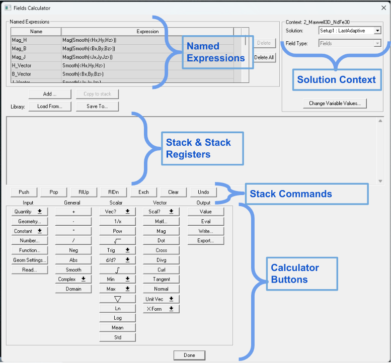
The Fields Calculator features a Calculator Stack, which can hold field quantities, functional or constant scalars and vectors, and geometries where field quantities need evaluation. You can manipulate these quantities using mathematical operations, integrate them over lines, surfaces, or subvolumes, plot them on various geometries, and export them for further analysis.
Calculating Average and Standard Deviation of the B-Field
To calculate the average B-field on a certain surface:
- Open the Fields Calculator
- In the 'Named Expressions' box, select 'B_Vector' and copy it to the stack
- In the 'Vector' category, select 'Mag'
- In the 'Input' category, select 'Geometry...'
- Select the geometry that you are interested in using for the calculation. This can be a model or non-model object.
- In the 'Scalar' category, select Mean
- Finally, select ‘Eval’ to see the result of the calculation.
The stack window should look like the following:
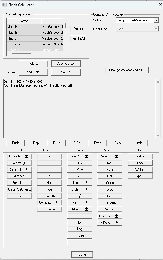
The top line gives us the value of the average B-field on the rectangle we created in the previous section. It is in the default B-field units, tesla.
To calculate the standard deviation, repeat the previous steps but instead of selecting 'Mean', select 'Std'.
Conclusion
In this guide, we've explored various techniques and methods within Ansys Maxwell for analyzing magnetic fields. We encourage you to experiment with these techniques and apply them to your specific engineering challenges.
For a more in-depth look into the material covered in this blog, please watch the associated YouTube videos!
Thank you for reading, and don't hesitate to reach out for further assistance or clarification.