
This post will demonstrate how to simulate a multi-conductor cable using Ansys 2D Extractor and use it in a circuit design simulated using Ansys Simplorer. Ansys 2D Extractor is an electromagnetic field solver which can quickly calculate the distributed RLCG parameters of cables and transmission lines over the desired frequency range. The cable parameters can be dynamically linked into a circuit model using an efficient reduced order model (ROM) representation. This allows the circuit simulation to accurately include the impacts of the frequency-dependent characteristics of the cable on the performance of the system.
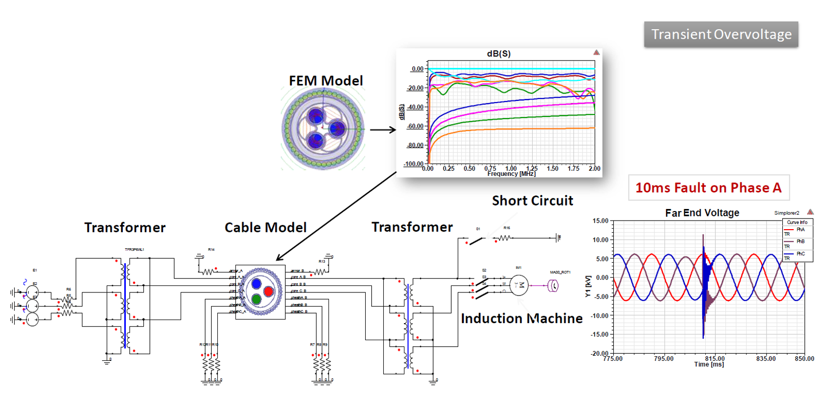
Let’s first look at several examples that show how these simulations work. The figure below shows a model of an armored multi-conductor cable used in a three-phase electric power system with an induction machine load. The detailed cable geometry is first simulated using the electromagnetic field solvers in 2D Extractor. This gives an accurate frequency response described in terms of distributed RLCG parameters or the equivalent S-parameters. Then the results from the cable simulation are dynamically linked into the system schematic which includes the power source, high voltage transformers, and the electromechanical load. The cable results are represented by a reduced order model which allows the system simulation to run very quickly. In this example, the simulation is predicting the effects of a transient short-circuit fault condition on one of the power system phases.
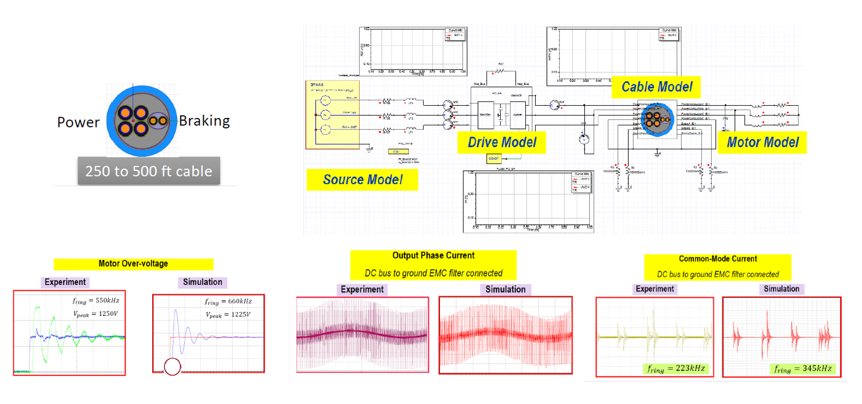
 A second example is the design of an AC drive system as shown in the image below. In this simulation, which is courtesy of Rockwell Automation, a shielded VFD cable with 4 power conductors and 2 braking conductors is first characterized versus frequency using 2D Extractor. Then the cable results are linked into the system model that includes the 3-phase source, the VFD drive with the rectifier and inverter, and the motor load. This approach gives good agreement between the simulation and measurement for the voltage and current waveforms.
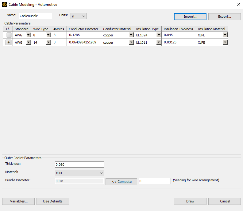
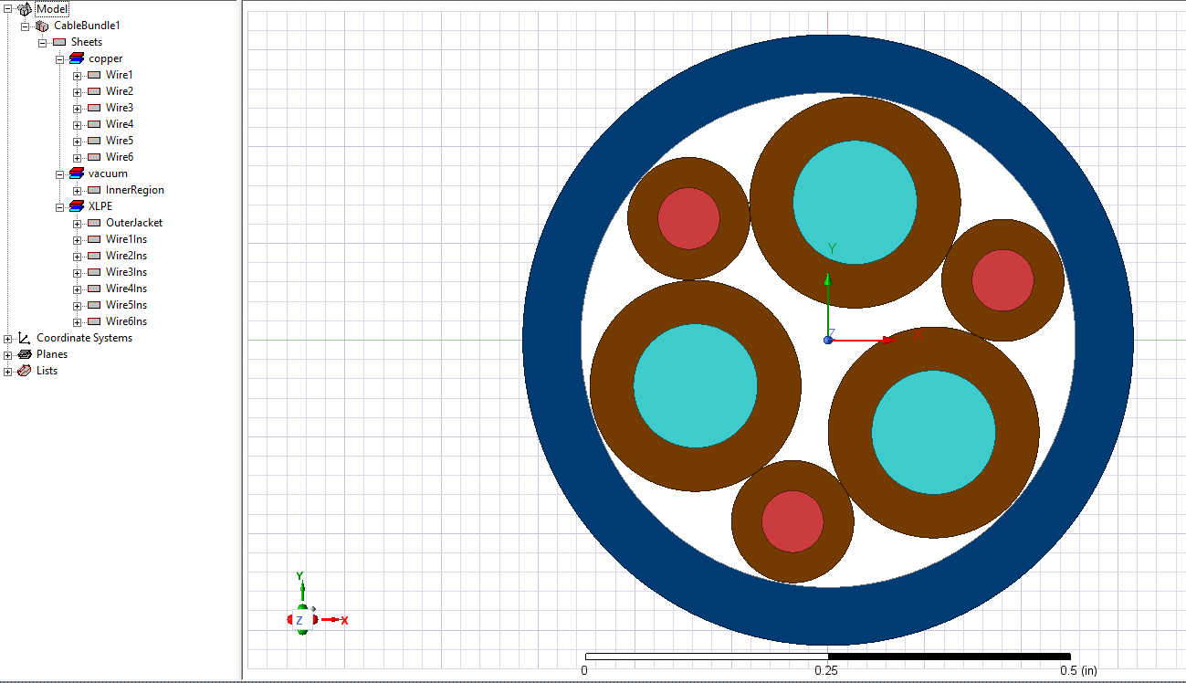
 To create these models, the first step is to define the cable cross-section geometry in 2D Extractor. This can be done by drawing the geometry, importing a DXF file, or using one of the Cable Modeling Toolkits included in 2D Extractor. The image below shows the Automotive Cable Bundle modeling toolkit which automatically creates the cable and assigns the material properties. For this example, we will create a typical multi-conductor cable with three 8 AWG copper conductors, three 14 AWG copper ground wires, and cross-linked polyethylene (XLPE) insulation and jacket. The resulting cable is also shown below.
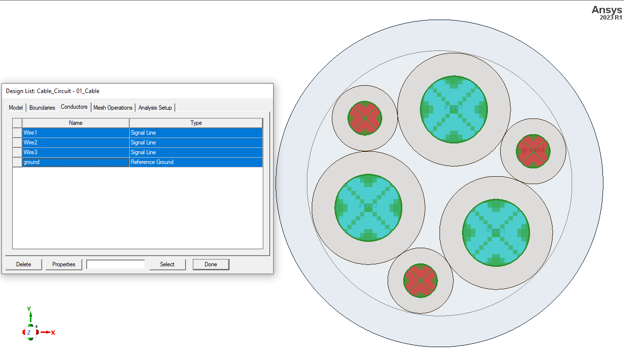
Once the cable cross-section has been defined and the model geometry has been created, the next step is to assign the signal and ground conductors. This can be easily performed by selecting each conductor in 2D Extractor and assigning the desired property. The results of this step are shown in the image below.
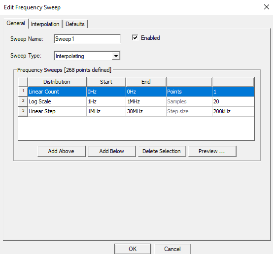
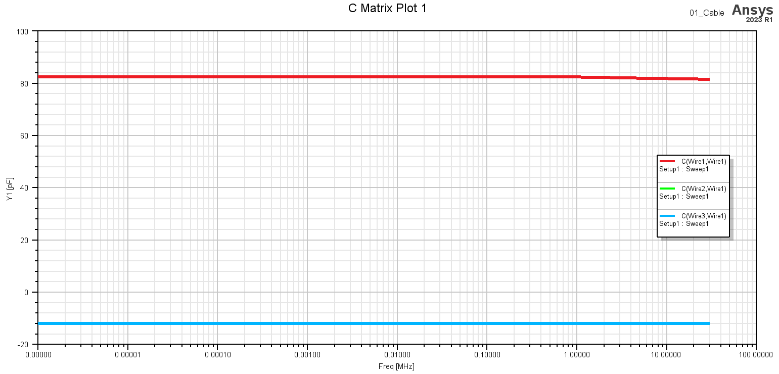
 The last step in 2D Extractor is to define the desired frequency sweep and solve the model for the RL and CG solutions. The frequency sweep should include sufficient resolution to capture the frequency-dependent behavior and cover the frequency range which includes the frequency content of the signal rise time that will be used in the circuit simulation. The frequency sweep type should be set to Interpolating to allow a fast solution. In this example, the interpolating frequency sweep is performed from DC to 30 MHz as shown below.
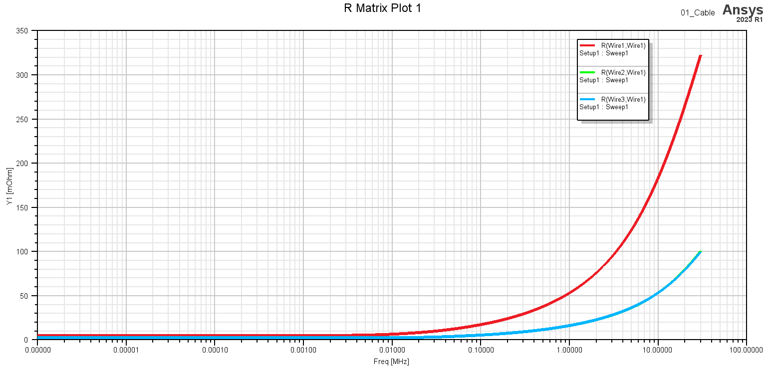
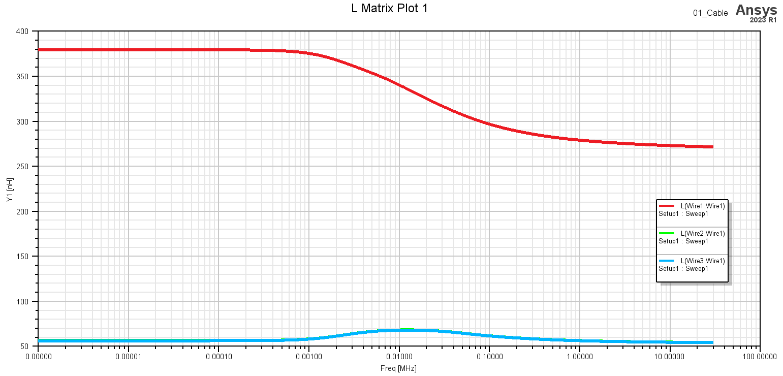
After the solution is finished, the distributed RLCG parameters can be viewed as a function of frequency. The plots below show resistance per meter, inductance per meter, and capacitance per meter of the cable conductors. The electromagnetic fields can also be plotted and animated for specified magnitude and phase excitations in the conductors.
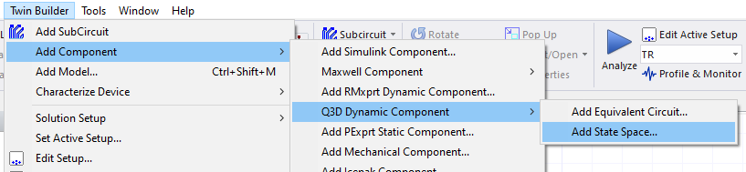
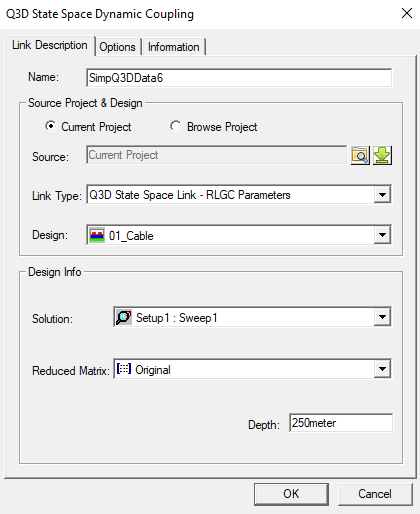
The cable results can be dynamically linked into the circuit using a reduced order model representation. This is done in Simplorer by selecting the menu item Twin Builder > Add Component > Q3D Dynamic Component > Add State Space. The State Space Dynamic Coupling menu allows the user to specify the Link Type, Design, Solution, and Cable Length. In this example, the RLGC Parameters link type and the frequency sweep solution is selected. The cable length is initially set to 250 meters and can be easily changed in the circuit model.
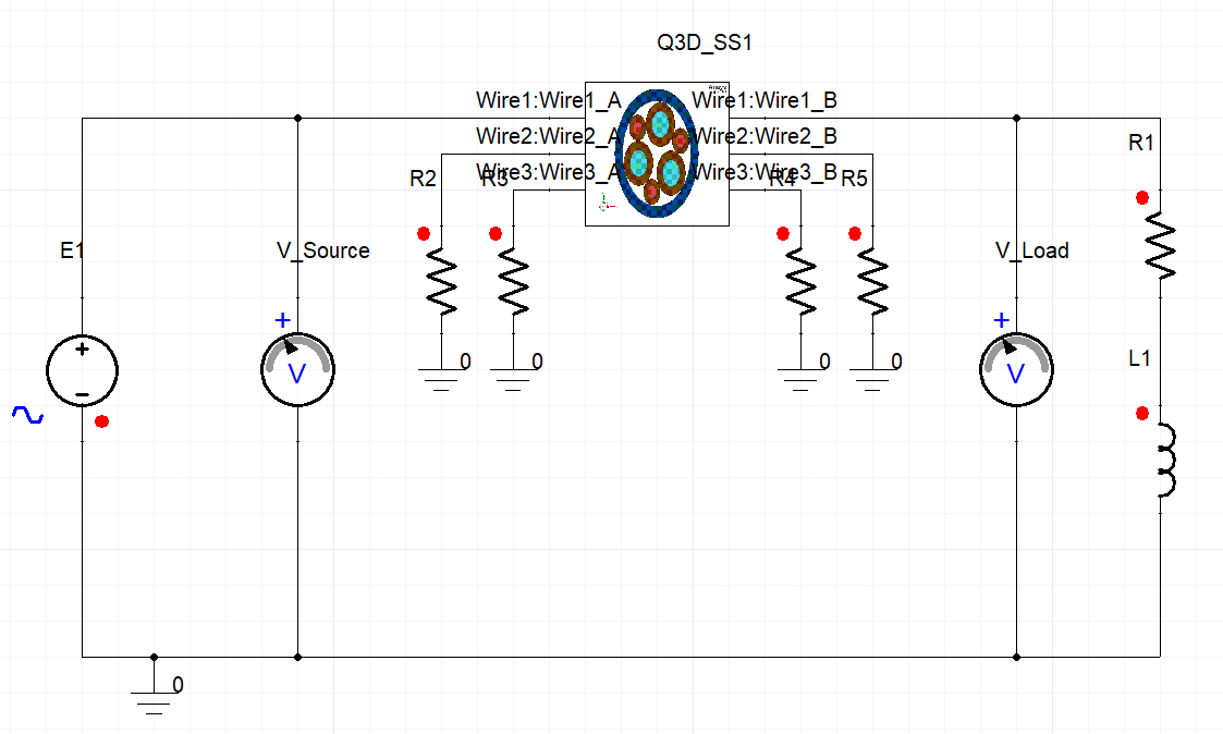
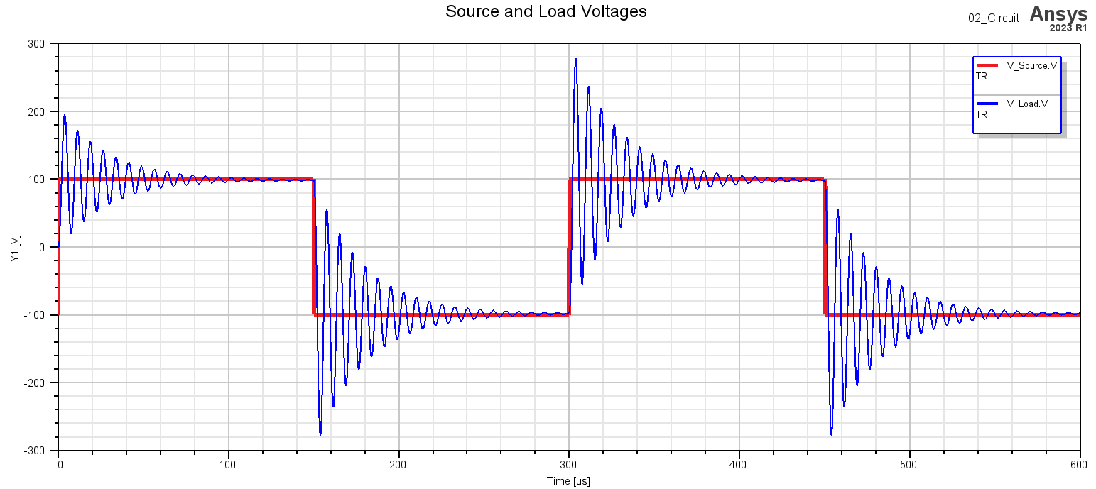
Once the cable is included in the Simplorer circuit schematic, it can be connected to the other components. In this example, the signal source is a trapezoidal periodic waveform (square wave) with a period of 300 us, amplitude of 200 Volts, and rise time of 100 nsec. A cable conductor is connected to a motor load represented by a series resistor and inductor and the other conductors are connected to ground through 1 MOhm resistors. Voltage probes are placed at the source and load to plot the input and output waveforms.
The transient simulation is performed for a duration of 600 us and a maximum time step of 10 ns. The maximum time step should be selected to ensure accurate sampling (>10 points) of the signal rise and fall times. The plot below shows the periodic input source waveform in red and the resulting load voltage waveform in blue. The cable ringing responses at the transitions of the input waveform can be observed. The ringing response corresponds to an underdamped sinusoidal waveform due to the reflected wave resulting from the cable and load impedances. This type of simulation can be used to characterize the transient response and peak voltage amplitudes for different cable types, lengths, and load impedance values.
A video showing the details of setting up the cable and circuit model can be viewed at the link below: