
Overview
Phased antenna array systems are used everywhere from defense radar applications to commercial 5G applications. Designing these antenna arrays involves complex mathematics that requires full wave simulation. Ansys HFSS full-field 3D electromagnetic simulation software can simulate a complex phased array antenna system in a reasonable amount of time and with low computation costs while considering the effects of complex excitations, environment (i.e., nearby antennas), and the platform on its performance.
One key feature of ANSYS HFSS is its antenna array unit cell simulation method, a powerful technique to approximate finite array patterns based on a single simulated antenna element. By leveraging this capability, engineers can quickly evaluate array performance, saving time and computational resources.
In this blog we will use the ANSYS HFSS tool to simulate the embedded antenna element radiation pattern based on unit cell analysis (infinite array simulation). This simulation method can be used to calculate the embedded element pattern to account for mutual coupling between the array elements and to create a more accurate overall array pattern.
Below is a brief overview of how HFSS can be used to simulate the embedded antenna pattern and a full demonstration is provided in the video link.
Embedded Antenna Element Radiation Pattern
The (active) embedded element pattern, is the radiation pattern of a finite array when only single element (often in the middle) is turned on while the other elements are terminated by its port impedance. The embedded element pattern takes into account the mutual coupling with adjacent elements. Therefore, embedded element pattern often differs from the single isolated element pattern or unit cell with periodic boundary condition. While the embedded element pattern is usually obtained from finite array simulation/measurement, a technique to obtain embedded element pattern from the unit cell analysis (infinite array simulation) is introduced.
Embedded Antenna Element Radiation Pattern Simulation
To simulate the embedded antenna element radiation pattern, the user first needs to setup a unit cell analysis using the lattice pairs boundary and steer the beam using the scan angles defined in the lattice pairs boundary setting. When steering the beam, we can look at the far field data in the unit cell analysis only in the direction of the scan angle (Theta_Scan, Phi_Scan). The pattern based on a regular Infinite Sphere is only valid at one point.
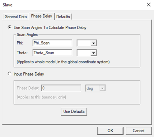
Figure 1. Parametric definition of Scan Angle in Slave boundary setting
The process of obtaining embedded element pattern includes the following steps:
1-Run parametric simulation of Theta_Scan and Phi_Scan to cover your desired scan volume.
2-Define an Infinite Sphere in sync with the Scan Angle. The proper definition of the Infinite Sphere is based on a Relative Coordinate System in which the z axis always points in the direction of Scan Angle. The specific settings for the Relative Coordinate System and Infinite Sphere are described below and shown in Figures 2 and 3.
Origin: 0,0,0
x-axis: cos(Theta_Scan)*cos(Phi_Scan) ,cos(Theta_Scan)*sin(Phi_Scan) ,-sin(Theta_Scan)
y-axis:-cos(Theta_Scan)*sin(Phi_Scan) ,cos(Theta_Scan)*cos(Phi_Scan) ,0cm
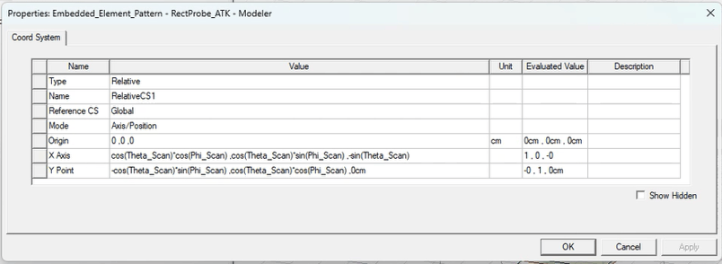
Figure 2. Definition of rotating Coordinate System (RelativeCS_Scan) aligned with Scan Angle.
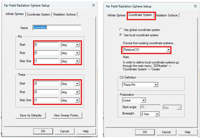
Figure 3. Definition of Infinite Sphere based on RelativeCS_Scan. Only one point on the z axis is chosen.
In the Far Field Report dialogue box, make sure to choose the proper Infinite Sphere in Geometry and Theta_Scan (or Phi_Scan) in Primary Sweep.
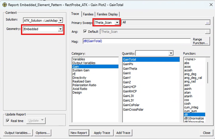
Figure 4. Important selections in the dialogue box for plotting RealizedGain are shown.
Realized gain is what typically considered when looking at the embedded pattern as it is the quantity that is affected by the impedance mismatch, since impedance changes as a function of scan angle.
This pattern can then be used to predict a finite array’s pattern through the method of pattern multiplication:
EFiniteArray=EEmbeddedElement X ArrayFactor
To fill in the rest of the pattern additional simulations need to be performed at different scan angles.
Note: Even though far field is only valid in the direction of Scan Angle, near field data (field within the unit cell) is valid at all locations. PML and FE-BI boundaries ae highly recommended here to improve the absorption and increase the simulation accuracy.
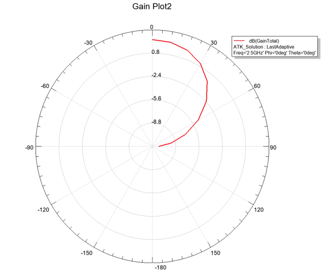
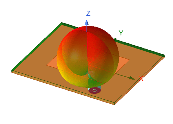
Figure 5. Simulated embedded element gain pattern.
The video link below shows an illustration on how to do these steps in detail, and the model shown is available in the downloadable resources.
Downloadable Resources