
When analyzing the electromagnetic compatibility (EMC) of a large, complex system like an aircraft, engineers face a significant challenge: how to accurately model an antenna's detailed radiation while simulating its interaction with the entire platform. Ansys offers a powerful solution by linking the high-frequency precision of Ansys HFSS with the system-level efficiency of Ansys EMA3D.


This hybrid workflow allows you to leverage a high-fidelity near-field antenna pattern from HFSS as a source in your EMA 3D imulation. In this guide, we'll walk you through the step-by-step process of exporting a near-field source from an HFSS antenna model and integrating it into an EMA 3D aircraft simulation to visualize its system-level impact.
Step 1: Exporting Near-Field Data from Ansys HFSS
The first stage is to generate and export the detailed field data from the source antenna model created in HFSS. In this example, we are using a slot antenna array.


Slot Array Geometry in HFSS (left), Plotted E-Field on XY-plane (right)


- Locate the Near-Field Boundary: In the "Project Manager" panel on the left, expand the project tree to find the Near Field Box located under the Radiation section.

- Export the Field Data: Right-click on the Near Field Box and select Compute Max Parameters... from the context menu. In the dialog box that appears, click the Export Fields button to proceed.
- Configure the Export Settings: This is the most critical part of the process. You must ensure the export settings are configured correctly to generate the compatible source files.
-
- Set Save as type: to Nearfield Data (*.nfd).
- Ensure the Export Points in: option is set to Local Coordinate.
- Crucially, check the box for Export near field descriptor (.and) file.

Step 2: Importing the Source into Ansys EMA 3D
With our near-field data successfully exported, we can now import it into our system-level EMA3D model.
- Open the EMC Plus Project: Launch Ansys Discovery and open the file you want to import the near field into. In this tutorial, the simulation domain, materials, and analysis probes have already been defined.
- Create a Near-Field Source: The simulation currently has no defined source. In the top ribbon, navigate to the EMA3D tab, find the Excitation section, and click on Near Field.

- Select the Descriptor File: In the pop-up window, change the file type filter to AND files (*.and) and select the exportfields.and file you generated in the previous step.
Step 3: Positioning and Configuring the Source
Once imported, the source must be positioned and scaled to fit its intended location—in this example, the radome on the aircraft's nose.

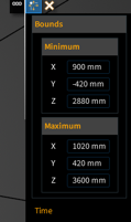
- Define the Source Bounds: In the source properties panel that appears, you will define the source's physical location using the Bounds settings. For this model, we'll enter the following coordinates to place the source correctly within the radome:
-
- Minimum: X: 900 mm, Y: -420 mm, Z: 2880 mm
- Maximum: X: 1020 mm, Y: 420 mm, Z: 3600 mm
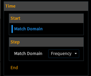 2. Set the Time Domain: Under the Time settings, expand the End option and click the button to Match Domain, which synchronizes the source timing with the overall simulation.
3. Confirm the Source: Click the "Ok" check mark in the model window to finalize the source setup. You will now see the new source listed under the Sources node in the Simulation Tree.
Step 4: Running the Simulation and Analyzing Results
With the high-fidelity source in place, we are ready to mesh, solve, and visualize the results.

Meshed F-16 Model.

- Mesh and Run: In the EMA3D ribbon, click Mesh to generate the simulation mesh. Once complete, click Start, and in the pop-up window, click Run to launch the solver.
Generate Field Animations: By creating animation probes, we can create useful visualizations for our results. To view the results, expand the Results node in the Simulation Tree, right-click on your results - Normal Electric Field, Normal H Field, and Surface Current Density- and select Generate Animation.
Normal E-Field, plotted in XZ Plane:

Normal H-Field, Plotted in XY Plane:

Surface Current Density:

Conclusion
By linking a detailed near-field source from Ansys HFSS into a system-level Ansys EMA 3D model, you can achieve a highly accurate and insightful analysis of platform-level electromagnetic effects. This powerful hybrid workflow enables you to identify and resolve potential EMC and EMI issues with confidence, ensuring the reliability and performance of complex electronic systems in their operational environments.
Ozen Engineering Expertise
Ozen Engineering Inc. utilizes its extensive consulting expertise in CFD, FEA, thermal, optics, photonics, and electromagnetic simulations to deliver outstanding results on engineering projects. We tackle complex challenges, including multiphase flows and erosion modeling, using Ansys software. Our team specializes in expert consulting and training in engineering simulations with Ansys, particularly Ansys Icepak AEDT, helping clients maximize its potential through scripting and automation.
We deliver customized engineering solutions in thermal management, fluid dynamics, and electromagnetic simulations. Our consulting, training, and support optimize performance and reliability across new and existing systems. Learn more at https://ozeninc.com.