
Explore the fascinating world of numerical dye washout using scalar transport equation in CFX through a detailed case study on blood flow dynamics in the aortic arch.
Introduction
Blood is not an ordinary liquid! Therefore, uninterrupted streamlined flow is critical for medical device applications due to a potential of thrombus formation because of flow stasis. In this blog, we demonstrated a residence time investigation method which numerically models dye washout using scalar transport equation. The geometry of a generic aortic arch with anastomosed ventricular assist device (VAD) outlet was utilized. Similarly, a representative generic boundary conditions were applied.
Theory of the Numerical Dye Washout Application
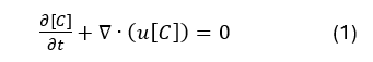
This method has recently been introduced to perform the VAD specific washout investigation1. The method relies on solving a scalar transport equation where the scalar demonstrates the dispersion of the dye. The dye concentration [C] was modeled solving a convection-diffusion-reaction equation in which the diffusion and the reaction (i.e. the source) were considered as zero (Eq. 1).
The fluid domain needed to be initialized with the dye concentration of 1, while the inlet dye concentration was 0. During the transient simulations, the dye from the inlet would be advected to the fluid domain, and time takes to clear initial dye would be analyzed.
Model Geometry and Flow Conditions
The image below shows the generic aortic arch geometry with anastomosed VAD outflow graft, which was considered as the “inlet” to this geometry. The outlets are the three branches and the main outlet.
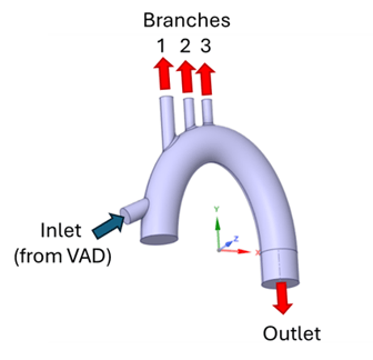
At the inlet, mass flow condition was applied which corresponds to the 5 L/min volumetric flowrate (a typical VAD flow). The branch outlets were also set as mass flow boundary condition with 20%, 10%, and 10% of the inflow for the 1st, 2nd, and 3rd branches respectively. Note that, these values are for reference only, and could vary depending on the application. Zero pressure condition was imposed to the outlet.
Setup
The Workbench environment was utilized with different modules as shown in the image below. The module for geometry generation and mesh was connected to separate CFX modules for steady-state and transient simulations. The data from steady-state simulation was used to initialize the transient one.
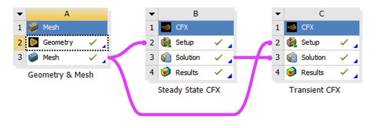
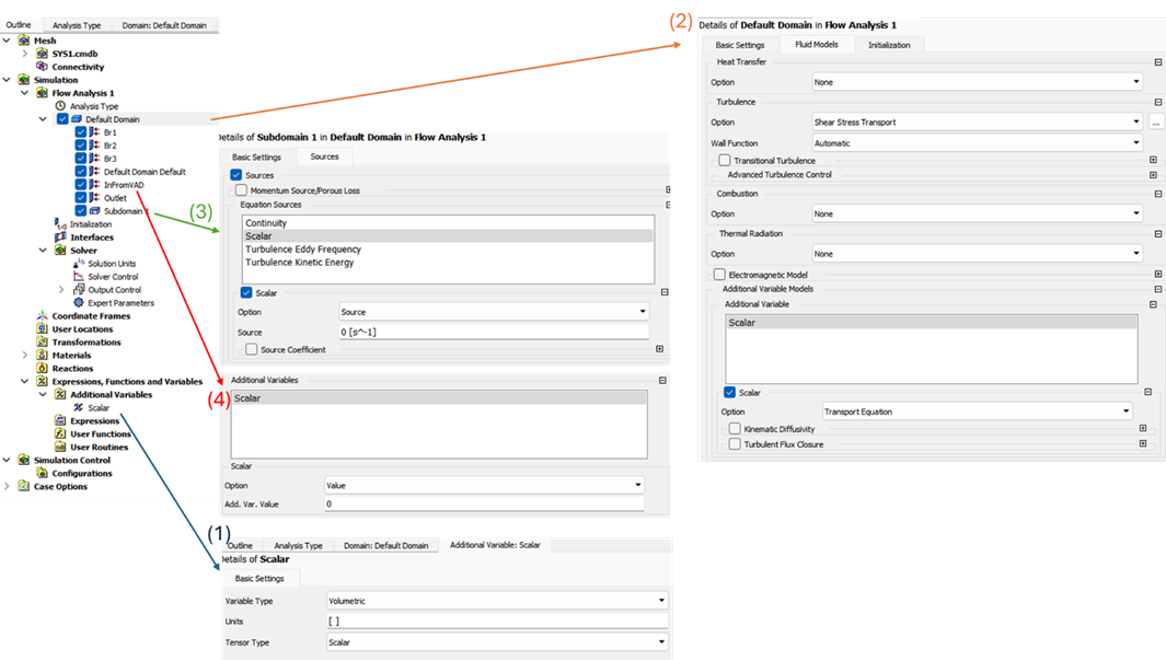
In this blog, the focus is given to the CFX components, therefore the geometry and mesh details are not demonstrated. Setting up the scalar variable is the same for both the steady-state and the transient CFX components: (1) Define a new volumetric “Additional Variable”, (2) Set “Transport Equation” for the scalar variable in the Default Domain, (3) Generate a Subdomain where the “0” source is defined, and (4) Define “0” value for the scalar variable at the inlet.
Since the steady-state simulation aims to generate data to initialize the transient run, only the fluids and the turbulence were solved in steady-state simulation. The scalar transport was initiated during the transient run.
Results
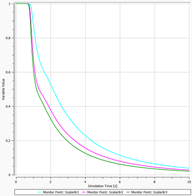
Results can be typically visualized with the scalar profiles and contours. The below image shows the profiles of the dye concentrations leaving all three branches. One can notice that, the concentrations did not change for about 1 second, then started to decline. Flow advection becomes effective after only a certain time which definitely depends on the boundary conditions.
The video below demonstrates this transient behavior with contour on a cross-sectional plane.
This method could be helpful to make a comparative analysis, and can be implemented to any problem where the residence time is an important parameter. It is demonstrated on an aortic arch with blood flow in this blog. However, it can be applied to any medical device associated with blood flow at many different settings.
Reference:
- Molteni, A, Masri, Z, Low, K, Yousef, H, Sienz, J & Fraser, K 2018, 'Experimental Measurement and Numerical Modelling of Dye Washout for Investigation of Blood Residence Time in Ventricular Assist Devices', The International Journal of Artificial Organs, vol. 41, no. 4, pp. 201-212.