
I. Mathematical Introduction to Self-Phase Modulation
A. Nonlinear Schrödinger Equation (NLSE):
The NLSE is a key equation in optics. It tells us how an optical pulse behaves in a medium that has both nonlinear and dispersive properties. The equation looks like this:
i ∂A/∂z + β2/2 ∂²A/∂t² + γ|A|²A = 0
Where:
- A denotes the complex envelope of the optical field.
- β2 represents the group velocity dispersion parameter.
- γ is the nonlinear coefficient.
- z symbolizes the propagation distance.
- t stands for the retarded time frame.
The term ( γ|A|²A ) within the NLSE is emblematic of the SPM effect. It conveys a fundamental concept: the modulation of a pulse's phase is intrinsically linked to its intensity gradient.
II. The Underlying Physics of Self-Phase Modulation
A. The Kerr Effect:
At the heart of SPM lies the Kerr effect. This effect describes how the refractive index of a medium dynamically adjusts based on the intensity of the light traversing it. The phase shift instigated by this change in refractive index can be quantified as:
Δϕ = γP₀L
In this equation:
- P₀ signifies the peak power of the pulse.
- L represents the length of the medium.
B. Spectral Broadening:
One of the things that happen when light goes through a medium is called spectral broadening. This is when the frequency spectrum of a pulse gets wider. This broadening can be seen as sidebands in the frequency spectrum. It's a clear sign of the interaction that's happening inside the waveguide due to the pulse's intensity.
III. Using Lumerical INTERCONNECT for SPM Simulations
Lumerical's INTERCONNECT software is a powerful tool for simulating optical circuits. It's especially good for looking at nonlinear effects like SPM. One of the things you can use in the software is the NLSE Waveguide (NLSE-WGD) element. It's designed to simulate how waveguides behave when there are nonlinear effects.
When you set up a circuit in INTERCONNECT, you can see the effects of SPM in different ways. For example, in the frequency domain, you can see the pulse's spectrum get wider as you increase the power. This is the spectral broadening we talked about earlier. But in the time domain, even as you change the power, the shape of the pulse doesn't really change. This tells us something about the balance of properties in the waveguide.
Figure 1 gives us a visual of the optical circuit inside INTERCONNECT. It's like a map that shows how different parts, like the source, monitor, and waveguide, are connected. By looking at this figure, we can understand the journey of the optical signal and where we can measure or change things.
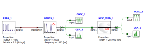
Figure 1: How the Circuit is Set Up in INTERCONNECT
Figure 2 is all about details. It shows how you can set different parameters in the waveguide element. Things like dispersion, the Kerr effect, the length of the waveguide, and even the amount of loss. Being able to control these settings means we can do simulations that are close to real-life situations.
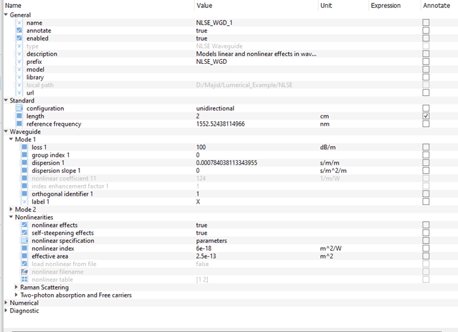
Figure 2: Setting Parameters in the Waveguide
Figure 3 lets us see the SPM effects when we use different power levels, but only in the frequency domain. It's like a snapshot of the pulse's frequency spectrum. As we change the power, the spectrum changes too. We can see it get wider, and this is the spectral broadening in action. It's a direct result of the nonlinear interactions inside the waveguide.
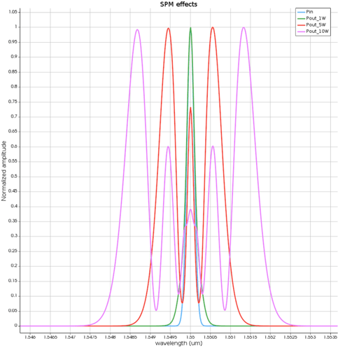
Figure 3: SPM Effects at Different Power Levels
For a hands-on guide on setting up an optical circuit in Lumerical INTERCONNECT and exploring the effects of Self-Phase Modulation, watch our video tutorial here: