SIwave: Unleash the power of the SIwizard solver

SIwave is a power integrity and signals integrity tool. SIwizard is the main tool for SI analysis in SIwave and is the subject of this blog.

SIwizard is used to study the signal integrity of RF, clock, and control traces. This tool allows users to do transient analysis, eye analysis, and BER calculations. Users can add IBIS and IBIS-AMI models to the TX and RX side. SIwave supports NRZ as well as PAM4 signals.

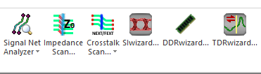
Figure 1: SIwizard solver 4^th icon 

SIwave should not be used to build PCBs. While this is possible, it is not the best way to use SIwave. SIwave can import the following types of CAD files:

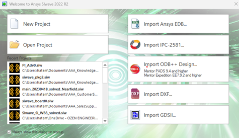
Figure 2: The import dialog box in SIwave

Users of Allegro and Altium can install Ansys EDB translator to produce EDB files. For users using Orcad, it is recommended that they use IPC-2581. People using Mentor Expedition should use ODB++ files. For Cadence users, generate BRD files and import them to the 3D layout. To do that, Cadence must be installed on the same computer, Extracta from Cadence must also be installed, and its location should be in the Path environment variable.

SIwave extracts lots of information from the CAD file, for example, the stackup, the materials, the components, and the nets. So, the model is ready to be solved.

1. Differential lines

Before launching the SIwizard, make sure that SIwave recognizes the differential traces. From Home, select the differential tab.

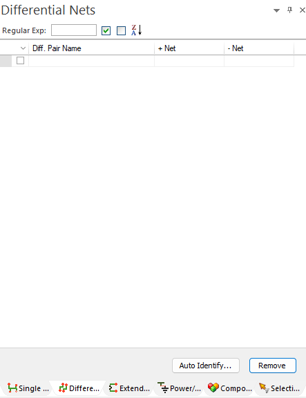
Figure 3: Differential nets tab

If it is empty, yet the user is sure there are differential lines in the model, then click on the auto-identify. SIwave opens a new dialog box and shows what notation it uses to recognize differential lines _P and _N. If it is correct, then click auto-identify. If different, the user has to change them in the dialog box.

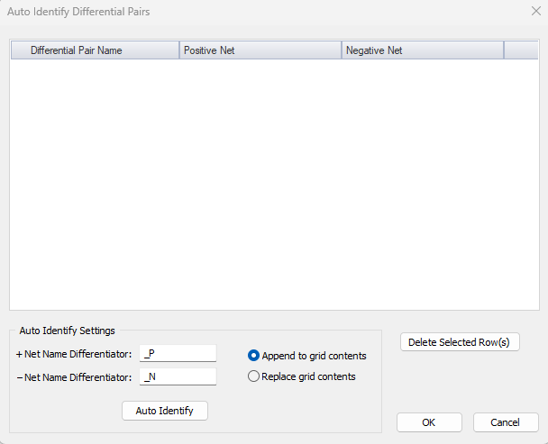
Figure 4: Differential nets auto-identify dialog box

After clicking auto-identify:

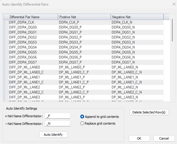
Figure 5: Differential nets tab after auto-identifying the traces

The user can also manually select two nets, move the mouse to the display area, right-click, and then select Create Differential Pairs.

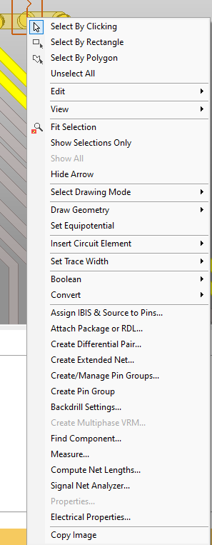
Figure 6: Alternative way to construct differential nets

If DC blocks separate the differential lines, the user can select to unite the lines first as extended nets and then create differential lines from them. Click first the extended tab, then select auto-identify

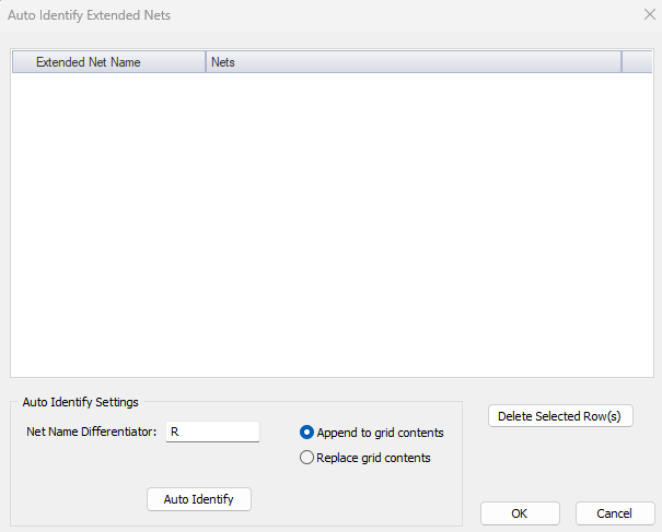
Figure 7: Extended nets auto-identify dialog box

SIwave displays a dialog box that shows that SIwave uses R to recognize extended nets. So any two nets with the same name but one with an extra R at the end will be combined.

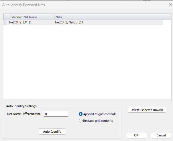
Figure 8: Extended nets auto-identify dialog box

Another way to create an extended net, especially if the net has more than two nets, is to enter a name for the extended net, then click edit:

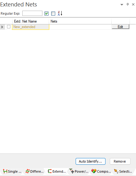
Figure 9: Extended nets tab

Then, you select the nets that can be joined from the list to create an extended net.

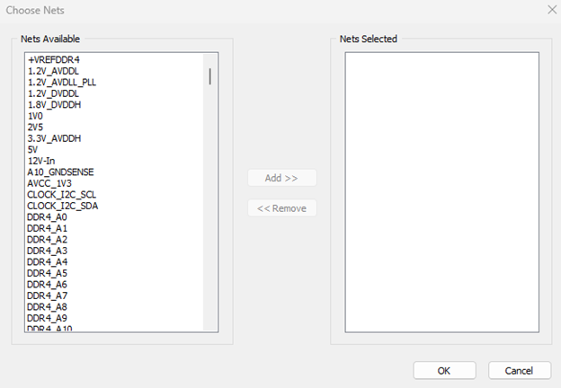
Figure 10: Extended nets: Select any nets to join

Another manual way is that the user can create extended nets by selecting single nets from the Single Ended Tab, moving the mouse to the display area, right-clicking, and then selecting Create Extended Net.

Figure 11: Alternative way to construct extended nets

Now, if the user wants to change the new extended nets to differential extended nets, then the user must follow the same steps explained before to create differential lines. The best way is to use the _P and _N notation with the new extended lines, auto-identify in the differential tab, and let SIwave do the combination.

2. Setting up the solver

Click on the SIwizard solver.

Before setting the solver, the user needs to understand what exactly SIwave will produce. It is going to create the circuit in the electronic desktop and do all the setup. Inside SIwave, the solver only calculates the s-parameters box. Yet it uses all the information the user provides to build and run the circuit in the Electronic desktop. Let us see how this is done.

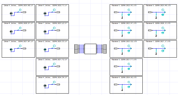
Figure 12: Schematic : Using Eyesource and Eyeprobe

Any process in SIwave: DC, PI, SI, or radiation starts by selecting a solver. Once a solver has been chosen, SIwave generates a dialog box that looks like a form. The user needs to check the form and fill in the missing information.

For example, SIwave populates the dialog box with all the existing traces in the model. One can select some of the lines or solve them all. Notice here that SIwave only selects the traces. Anything classified as a power plane SIwave does not put it in the table.

Now, in the table, there are four categories: Single, differential, extended, and extended differential. Make sure to check the four categories and select the traces to do SI on them. Select to use eight single lines for simplicity.

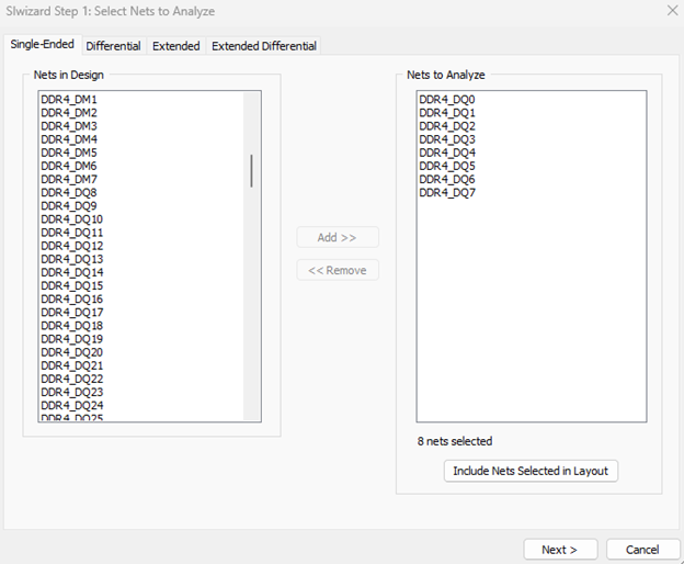
Figure 13: Select traces

Select next to display the Set Drivers/Receivers dialog box. What is the meaning of these columns?

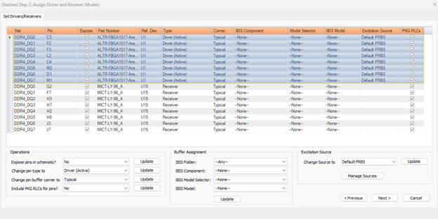
Figure 14: Define excitations: Drivers and Receiver

• The first column is the name of the single-ended net. Even if the lines are differential, SIwave still displays the single-ended names.
• The second column is the pin name in the component mentioned in the fifth column, Reference Designator.
• Column three, Expose, means that the user wants SIwave to put a port at that end of the trace. Usually, only the ends connected to a discrete device or an integrated circuit are exposed. That does not mean that it cannot be exposed if the ends are connected to an R, L, or C.
• Column four is the part number of the column 5. So, the same part could be used in the circuit many times. Each one has its own Reference Designator, mentioned in column 5
• Column six, where the user specifies if this end is a driver or a receiver if the expose option is checked. On one end, select the Driver; on the other, select the Receiver. This information goes to the circuit. SIwave does not use this information.
• Column 7 is the corner, i.e., if the user adds an IBIS model. These are usually related to temperature and supply voltage conditions. SIwave selects the correct data set based on your selection here: Max, Min, …
• Column 8 is the IBIS model on the TX or RX side. If one is selected, the user must also specify options in columns 9 and 10.
• Column 12 is the PKG RLC. This is important if you are using IBIS models and would like the RLC of the package in the IBIS model to be included.
• Column 11 is the signal. The user can select PRBS, clock, step, or random RPBS. Right below this column, there is the excitation source box. Click on Manage sources. Notice the four options.

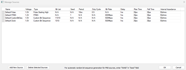
Figure 15: Define signals

For each, the user needs to specify

• the voltage for the DDR4 it is 1.2Volt
• the type of signal,
• the bit list if it is a custom PRBS or a clock,
• the seed (used when defining Bytes),
• the period,
• the duty cycle, the ratio between the 1 and 0 durations,
• the bit rate,
• the delay,
• the rising time, in the DDR4-3200 it is 35ps
• the fall time, same as the rising time, and finally
• the input impedance of the Driver.

Notice the note that if the user wants a random bit sequence PRBS, enter RAND in the seed field.

The user can also add more sources, but they must be one of the four types: Pulse PRBS, pulse starting high, pulse starting low, or random bit sequence. So, one can add a PRBS signal with different data rates or rising time.

Returning to setting the Driver and the Receiver. The information about the signal also goes into the circuit in the definition of the eye source and eye probe.

If the user selects more than one row, the options at the bottom get activated. So now, the user can change more than one row in one click.

After being satisfied with the choices, click next to assign the receivers the proper terminations:

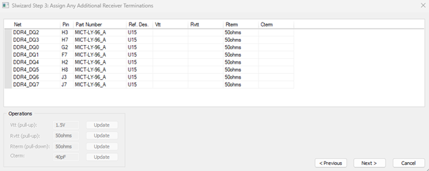
Figure 16: Define Receiver setup : Vtt pullup voltage.

• Column one is the race name,
• Column two is the pin numbers,
• Column three is the part number,
• Column four is the Reference designator,
• Column five is the Vtt used with SDR applications, usually equal to VddQ/2. It is the pull-up voltage,
• Column six is the Rvtt used with SDR applications, and it is the pull-up resistor,
• Column seven is the termination resistance,
• Column eight is the termination shunt capacitance.

Like in every dialog box in SIwave, the lower section gets activated if the user selects more than one row.

Click next.

The following dialog box is the power plane setting. In this dialog box, the user adjusts the power nets feeding the components used in the traces at the input or at the output. The user usually does not need to change anything because SIwave fills up all the entries.

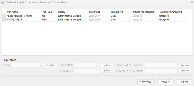
Figure 17: Power planes setup

The last step is the solver.

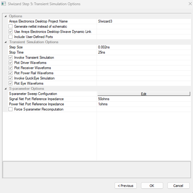
Figure 18: Solver setup

• Enter the name of the solution in the first line: SIwizard with no IBIS models.
• In the second line, if selected, SIwave would not generate the schematic if it is selected.
• Row three, if selected, SIwave generates the schematic in the electronic desktop.
• Row four, if the user wants SIwave to include user-defined ports. These are ports that the user generated outside the SIwizard, and wants them to be included in the s-parameters. Something like access points of power plane ports.
• Row five is the step size, and this is a function of the shortest rising time; 1/5 is the maximum
• Row six is the Stop time; usually, it is a function of the longest structure. Rows five and six are used in the definition of the transient solver.
• Row seven forces the transient solver in the electronic desktop to solve
• Rows eight, nine, and ten are for plotting the results.
• Row eleven is to invoke the quick eye solver in the electronic desktop that generates the eye plot.
• Row twelve is to plot the eye after finishing the quick eye solver. Again, lines eleven and twelve are used in the circuit.
• Row thirteen is for the s-parameter solver inside SIwave. SIwave only does the s-parameters solving. The transient and the quick eye are done in the electronic desktop.
• Rows fourteen and fifteen are to confirm the reference impedance of the ports for the s-parameters.
  .

In row thirteen, if the user clicks edit, the s-parameters solver that was explained in the SYZ solver pops up. Please refer to the video of the PI solver for more information about the setup here. One should notice that the maximum frequency is related to the min Rise/Fall time. Also, notice that more options exist if the user clicks the other solver options.

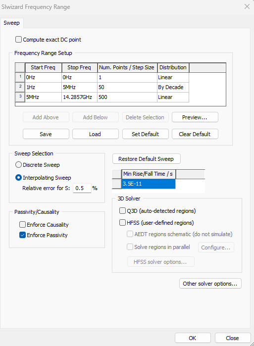
Figure 19: S-parameters solver setup

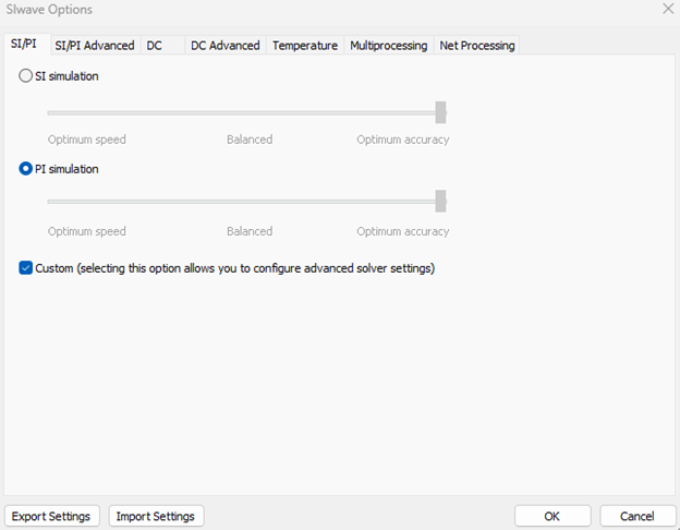
Figure 20: Accuracy versus speed setup

Go back to the transient solver setup, and press OK

The same steps are repeated after adding IBIS models and naming the solution SIwizard with IBIS models. This way, the user can see the difference between the two.

3. Solutions
   • Transient solution

The first result is from the transient solver. The transient solver plots what the user asked for, the voltage at the Driver and at the Receiver, of course, for the selected traces. Notice in the plots that the p-p voltage is half 1.2Volt. This is because the circuit acts as a voltage power divider between the source and the load. So, in the setup, always put two times the voltage.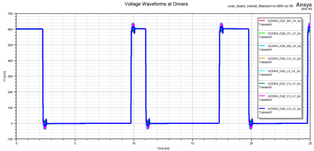

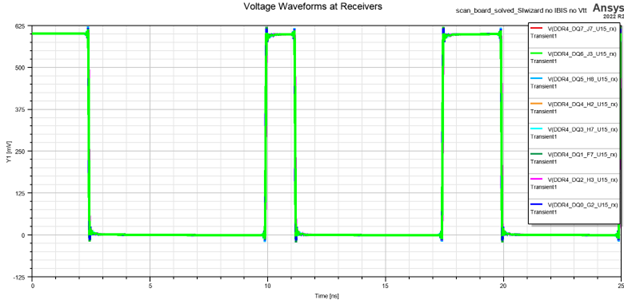
Figure 21: Transient response PRBS signal

If the user does not have the license to do eye analysis, the user can always use the transient solver to produce an eye plot. After doing the transient, select Results->Create eye diagram report->Rectangular plot-. Keep the solution on the Transient, but change the unit interval to the interval of one bit.

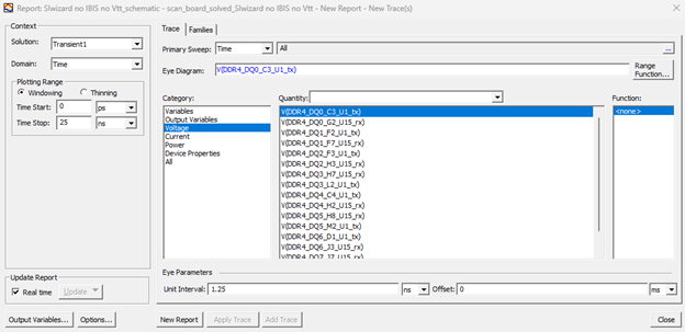
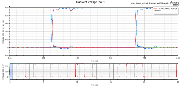
Figure 22: Producing eye plot from transient solver

•  Quick Eye solution

The second result is coming from the Quick Eye. The user can plot three types of eye plots from the quick eye solver. Notice that one needs to select the probe to plot.

• Results->Create Eye Diagram Report->Rectangular Plot

• • Can add the eye information and measures
  • Is a function of the time interval
  • Displays the shape of the signal for ten times the period specified in the transient solver.
  • Add a Mask: Double-click the graph, select Mask, Edit, Edit again, and enter the mask in voltage and time.
    
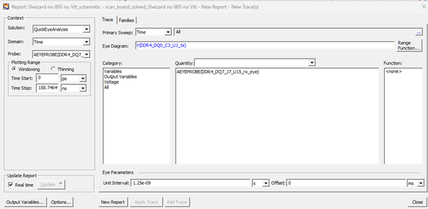
    Figure 23:  Results->Create Eye Diagram Report->Rectangular Plot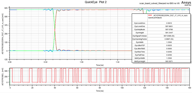
    
    
    Figure 24:  Eye Plot: Results->Create Eye Diagram Report->Rectangular Plot
    
    
• Results->Create Eye Diagram Report->Stacked Eye Diagram Plot:
  • Can add the eye information and measures
  • Is a function of the time interval
  • Cannot add a mask
  • Eye measurements are generated automatically on the side

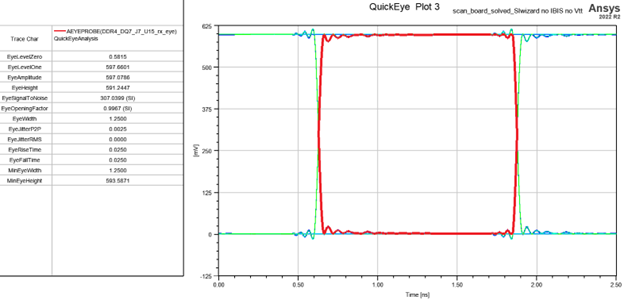
Figure 25:  Eye Plot: Results->Create Eye Diagram Report->Stacked Eye Diagram Plot

• Results->Create Statistical Eye Diagram->Statistical Eye Plot
  • Can add the eye information and measures
  • Is a function of the unit interval
  • Can add all eye information
  • Can add a mask: Double click the graph, select Mask, Edit, Edit again, and enter the mask in voltage and unit interval.
  

   

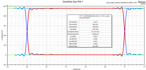
  Figure 26:  Eye Plot: Results->Create Statistical Eye Diagram->Statistical Eye Plot

• Verify Eye solution

The third result is available if the user adds the Verify Eye solver. Then, the user can plot the bathtub results. The user can determine the eye width at a specific BER from the bathtub. Just select the y-marker and set the y-value to the required BER.

Results->Create Standard Report->Rectangular Plot->Bathtub

• Can add a Y-marker to detect the eye-opening at any level (the Y-axis is the BER level)
• Can also add a limit line
  
   

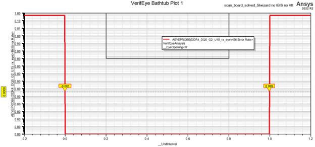
  Figure 27:  Eye Bathtub from VerifyEye

• Vtt models

Add the Vtt and Rvtt to the setup. As said, this setup is used when you have no IBIS models and the traces are for SRD and not DDR. The circuit is as shown below.

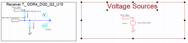Figure 28: Schematic : Using Eyesource and Eyeprobe and Vtt circuit

And these are the results. Completely different.

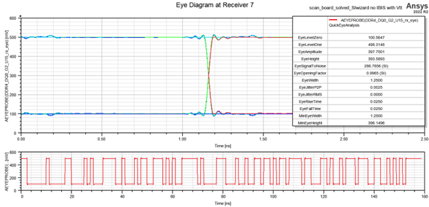Figure 29:  Eye Plot: Results->Create Eye Diagram Report->Rectangular Plot

• IBIS models

Adding the IBIS model, the circuit changes to include the IBIS components in the Ansys circuit. Notice that with these components, the user still needs to have the eye source and eye probe.

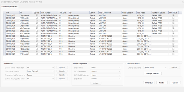Figure 30: Entering the IBIS model in the excitation definition

The eye source and the eye probes are there if the user wants to use the Quickeye and the Verifyeye solver. However, the setup inside the Eyesource is wrong because it is not used. All the information about the signal comes from within the IBIS model.

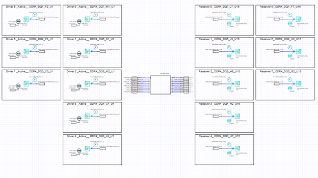
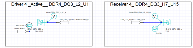Figure 31: Schematic : Using IBIS models

Open the dialog box of the IBIS model.

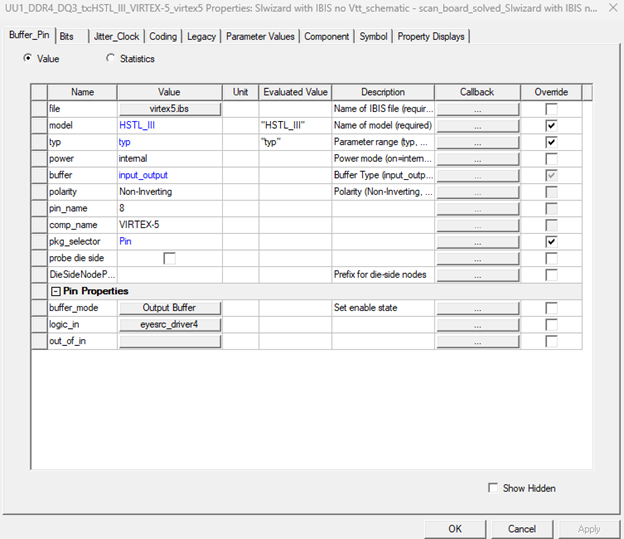
Figure 32: IBIS model dialog box

• The file name
• The model used in the file name, in this case, select the HSTL (high-speed transceiver logic)
• Type which is the corner: Is it typical, min, max, or anything else? These are the options inside the IBIS file.
• Power is coming from the IBIS file itself, not from the Eyesource (internal)
• Buffer: input Rx, output Tx, or input-output. Documented in the IBIS file, the user cannot change it. In the case of input-output, then in the buffer_mode below, the user must specify which one: input or output.
• Polarity, inverting or non-inverting
• Pin-name in the file
• Component name
• Package selector (Pin/Package/None): In the IBIS file, there are two sections, [Package] section and [PIN] section. Package has the traditional R_pkg, L_pkg, and C_pkg. The Pin one is a list of pin names
• Probe die side:
• Die Side Node Prefix: If the die pins have any prefix in their names.
• Buffer_mode: Used when the buffer is input-output.
• Logic_in for the user to enter the name of the Eyesource pin. If it is set to internal, then the user needs to go to the Bits tab and enter the definition of the signal.
• Out-of-in:
  
  
  
  
  
  

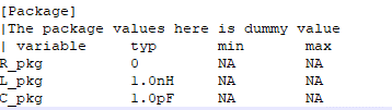
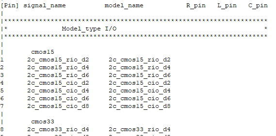
Figure 33: IBIS file: [package] and [pin] sections

If the user selects to use an internal source instead of the eye source, then a dialog box similar to the one in the eye source appears in the Bits tab.

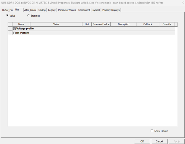
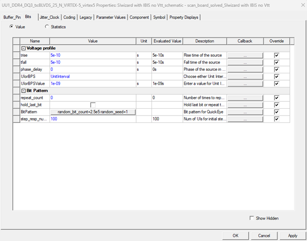
Figure 34: Bits tab with and without Eyesource

If the IBIS file has more options, then activate show hidden, and the user can have more items to select.

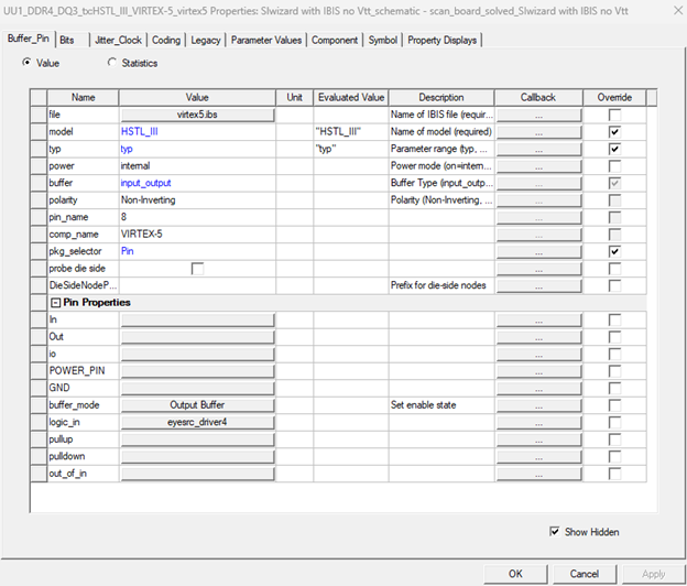
Figure 35: IBIS model dialog box with more options

And these are the results:

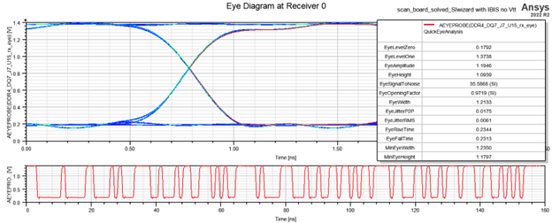
Figure 36: With IBIS models: Results->Create Eye Diagram Report->Rectangular Plot

There will be a session about the IBIS models in AEDT electronics. We will talk more about all the options.