
SIwave is a power integrity and signals integrity tool. CrosstalkScan is one of the most essential tools in SIwave and is the subject of this blog.
Zoscan was explained in another blog and video. Zoscan highlights defects in the traces. It calculates the impedance along the path. Also, in another blog and video, the TDRwizard was discussed, and the TDRwizard's main job is to identify discontinuities or any defects in the transitions in all traces. The crosstalk scanner's main job is to identify any fault in the grounding around the traces, including the vias. It highlights areas where the traces are not well isolated and protected.
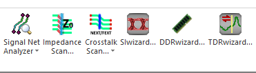
Figure 1: Zoscan solver 4th icon from the left
SIwave should not be used to build PCBs. While this is possible, it is not the best way to utilize SIwave. SIwave can import the following types of CAD files:
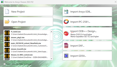
Figure 2: Import dialog box in SIwave
SIwave extracts lots of information from the CAD file, for example, the stackup, the materials, the components, and the nets. So, the model is ready to be solved.
- Crosstalk Solver – Frequency Domain.
Click on the Crosstalk Scan solver and select the frequency domain option.
Any process in SIwave: DC, PI, SI, or radiation starts by selecting a solver. Once a solver has been chosen, SIwave generates a dialog box that looks like a form. The user needs to check the form and fill in the missing information.
For example, SIwave populates the dialog box with all the existing traces in the model. One can select some of the lines or solve them all. SIwave uses advanced techniques that can solve all the lines very fast.
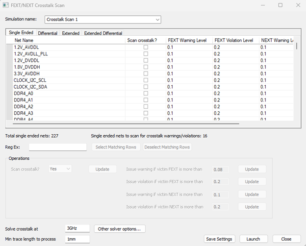
Figure 3: Crosstalk – Frequency Domain dialog box
Notice here that SIwave only selects the traces. Anything classified as a power plane SIwave does not put it in the table.
Now, in the table, there are four trace categories: Single, differential, extended, and extended differential. Make sure to check them all. For each trace, one needs to specify the limits, warning, and violation limits. These numbers help to zoom in on the bad and worst areas later.
So what is FEXT? And what is NEXT? The SYZ-solver provides the total crosstalk seen from the ports of other traces when a sinusoidal signal is injected in the aggressor trace. There are two types of crosstalk: the far-end crosstalk and the near-end crosstalk. The far-end always goes in the same direction as the wave propagation. The crosstalk from the different sections arrives simultaneously at the far-end port of the victim. While in the near-end crosstalk, the wave has to reverse its direction. The crosstalk from the different sections does not arrive at the same time at the near-end port of the victim.
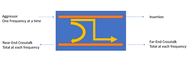
Figure 4: Near-end and far-end crosstalks
In the crosstalk scan solver, the signal is assumed to be a step response instead of the sinusoidal signal—the traditional signal in any digital communication. Then, one observes the signals at the victim's ports. The signals seen at the far-end and near-end are well known, but not their amplitudes. For the far end, it is FEXT times Vi, and for the near end, it is NEXT times Vi. FEXT and NEXT are related to the mutual capacitance and the mutual inductance with the formulae shown below.
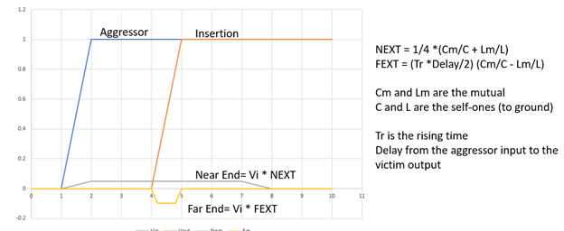
Figure 5: FEXT and NEXT definition
In SIwave, the FEXT is defined in a slightly different way:
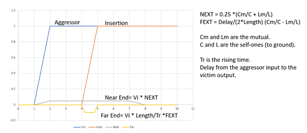
Figure 6: FEXT and NEXT definitions in SIwave
And this is the more detailed formulae if you are not happy with the simplifications:
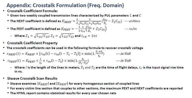
Figure 7: FEXT and NEXT definitions in SIwave in details
Back to the setup:
Use the "Other solver options" button to decide on the accuracy of the solution. Three options: optimum speed, balanced, or optimum accuracy. Start with the balanced, and after one solution, one can decide what to do for the next ones.
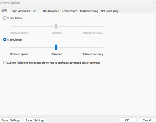
Figure 8: Advanced options SI/PI tab
There are more advanced options in the SI/PI Advanced:
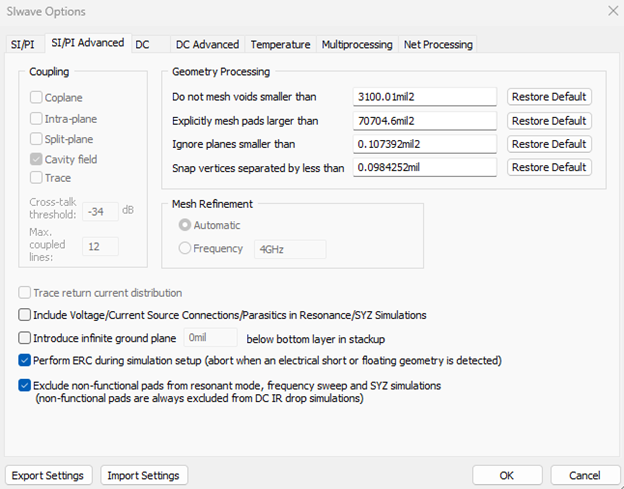
Figure 9: Advanced options SI/PI Advanced tab
If the Custom button is activated, then the user has more options in the SI/PI Advanced tab.
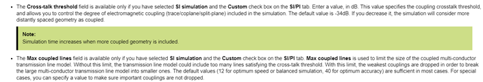
Figure 10: Crosstalk threshold definition
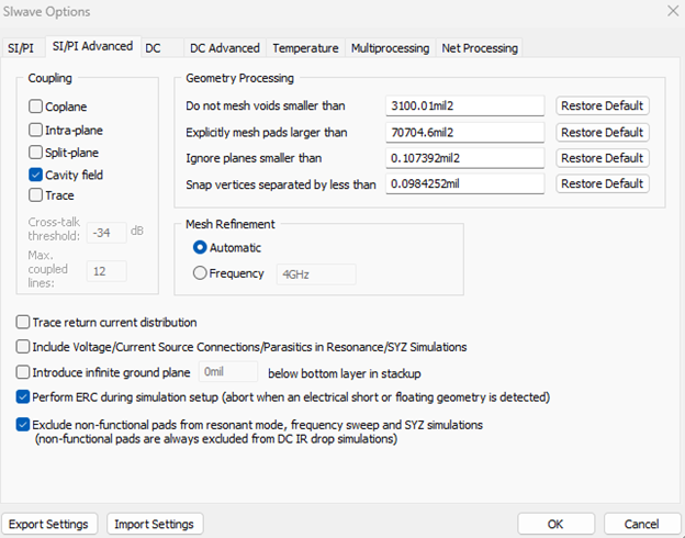
Figure 11: Advanced options Advanced SI/PI tab with more options
One can control the meshing and force the solver to mesh at a specific frequency for the crosstalk scan. The user can also change the crosstalk threshold and the maximum number of coupled lines.
Click on the temperature tab to select another temperature that will affect the conductivity of the traces. Notice here that one can import the temperature distribution from Icepack to the model. Just specify the Icepack file name and the simulation name in that file.
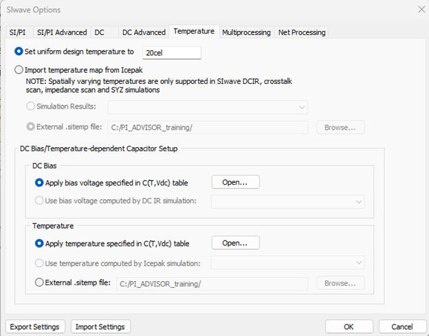
Figure 12: Advanced options temperature tab
Select Multiprocessing to select how many cores to use and the percentage of RAM to use.
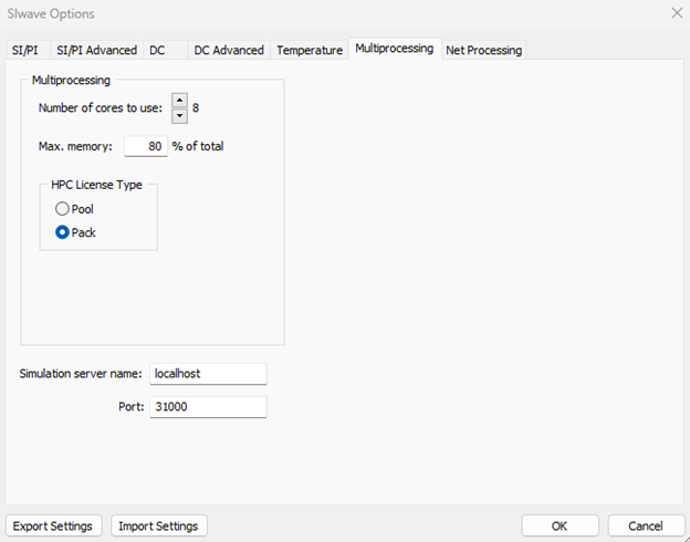
Figure 13: Advanced options Mutliprocessing tab
Going to the Net processing, more options. The user can add more nets, like the ground and power nets, to the simulation, of course, if the user wants to see the crosstalk between the traces and powerplanes or between the powerplanes themselves.
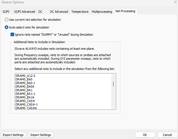
Figure 14: Advanced options Net Processing tab
Before launching the solver, name the solution because you will need to do many solutions. For example, here, call it FrequencyDomain_3GHz.
Examining the solution:
- Crosstalk distribution
The first result is the crosstalk coefficient along each path. The scale on the side shows the worst crosstalk level coefficients. Display the near-end or the far-end crosstalk for all the traces. The proper way to use these values is first to identify which trace is getting unacceptable crosstalk, near-end or far-end, then use these plots to locate the weakest sections and try to isolate them better.
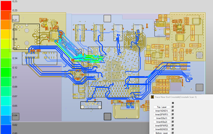
Figure 15: Crosstalk level along each trace – NEXT values
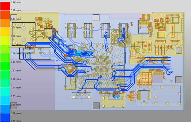
Figure 16: Crosstalk level along each trace – FEXT values
- Zoom in and hover the mouse over any line to see the values at any point. Notice that it tells if this is a SE or a differential trace.
- Change the scale, double-click the barcode, and modify the scale. Select a log scale if there is a significant variation.
- Select which layer to display.
- If the user is examining the crosstalk and wants to know which line is this? Activate the trace option in all layers. Now, the user can see the original nets, zoom in, and identify the net.
- Violations plot
The second result is even better because the solver identifies where the crosstalk crosses the warning and violation levels. This way, the designer can zoom faster on bad areas. The problem could be poor grounding, insufficient vias, bad transitions, small separation, and/or large layer thickness.
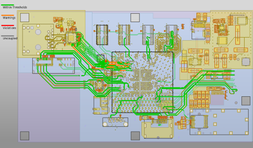
Figure 17: Crosstalk violations
- Coupled Structures
From the crosstalk results, SIwave detects which sections of a trace cannot be considered single but rather coupled to other lines. The colors in the plot are all relative. The plots are a function of the setup. We define the crosstalk and the number of coupled traces in the setup.

Figure 18: Coupling conditions

Figure 19: Coupling degrees in each section of all the traces
- Generate Report
SIwave can also put all the information in a table. This table summarizes in detail all the findings.
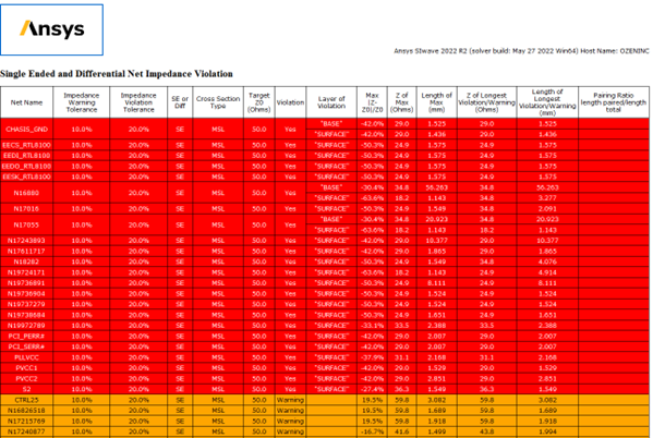
Figure 20: Summary of the crosstalk results
- Modify traces.
To modify any trace, click on it, select the Centerline Edit, then change the width and the coordinates of the center line.
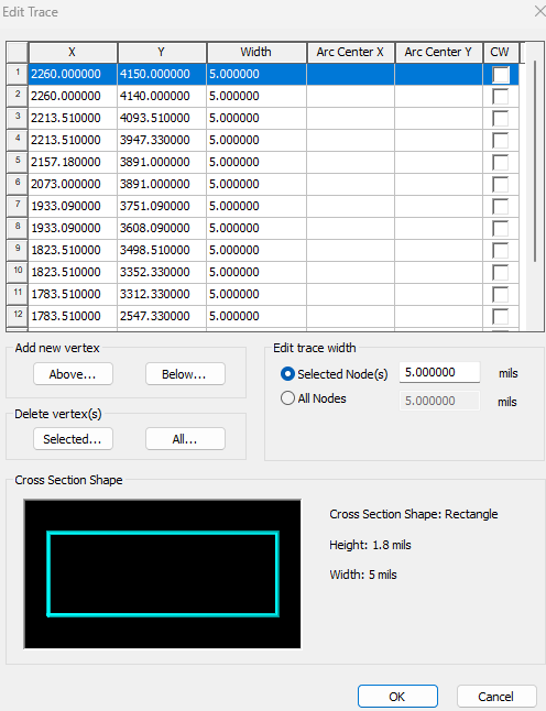
Figure 21: How to modify a trace
- View the profile.
View the profile.
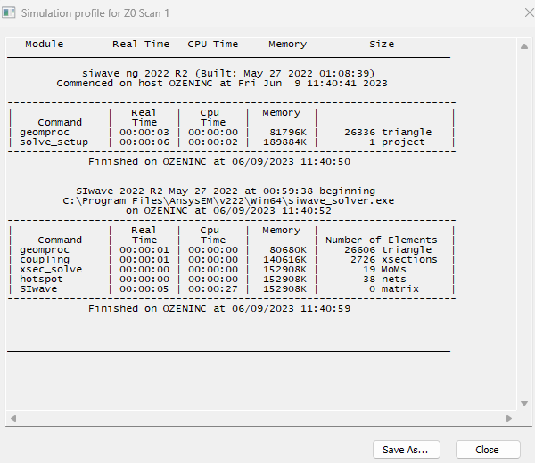
Figure 22: Profile
- Crosstalk Solver – Time Domain.
Select the Crosstalk Scan solver and select the time domain option. Again, another dialog box. SIwave populates the left column with all the traces. Notice all the tabs for the single and differential. Select the lines to analyze and move them to the right column. Press Next.
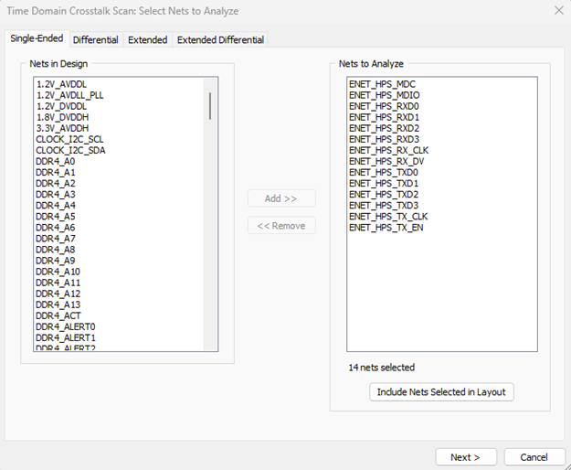
Figure 23: Crosstalk – Time Domain dialog box
The time domain one is like a TDR analysis. It sends signals from one side and reads the signal on the other ports. So, one needs to specify the rising time and voltage of the signal used on each trace. The rising time defines the bandwidth of the signal. After filling the table, we start the solver.
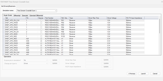
Figure 24: Enter the rising time and voltage level
Examining the solution:
- Trace to Trace Crosstalk
The first result is the crosstalk between any two traces. If one clicks on any bar, SIwave will display the far-end and the near-end crosstalk voltage response. On the left bar, one can select to display the far-end or the near-end in the bar plots. The plot under the bar plot always has both curves.
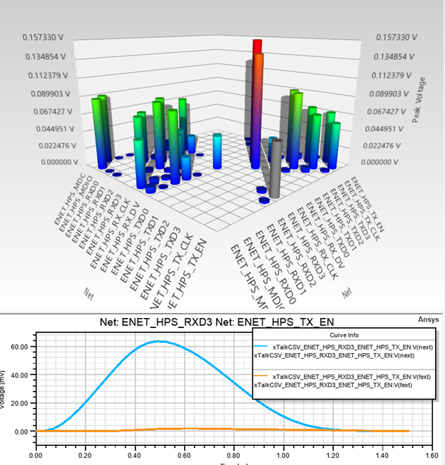
Figure 25: Crosstalk between any two traces (Bars) and the TDR along one trace (Curve plot).
The user can also add the input and output signals on the aggressor line. You can also plot many crosstalk for different traces. The users do that for comparison.
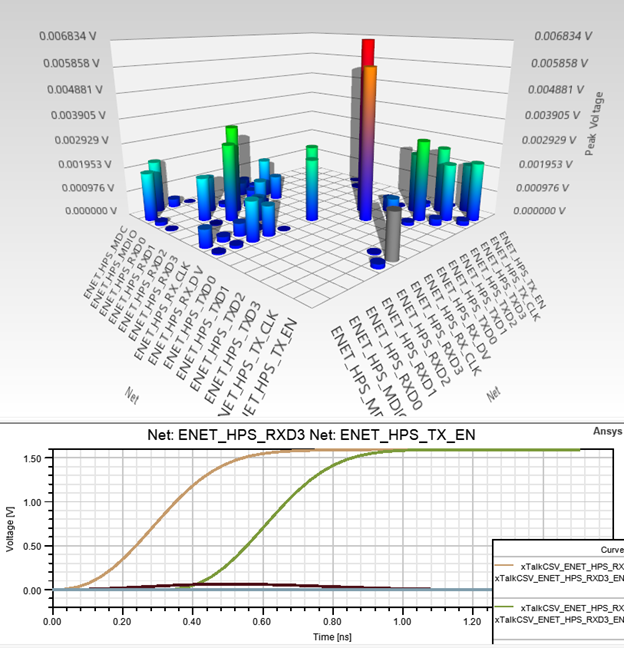
Figure 26: Crosstalk between any two traces (Bars) and the TDR along one trace (Curve plot).
So, the time domain bar shows the worst crosstalk voltage. It also plots the spread of the crosstalk along the traces. That is why the curves are plotted versus time. The time here is equivalent to the physical distance. The time domain results allow the designer to understand the expected crosstalk based on the rising time of the signals used in operation. In contrast, this information is hard to realize from the s-parameters.
- Crosstalk distribution along the traces
As in the Frequency domain option, the time domain can predict the location of the worst possible crosstalk along any trace. But in the time domain, SIwave displays the summation of all the voltages from all the other lines. This plot highlights the traces with weak protection. Maybe the magnitude does not say much, but the colors can help the designer identify areas needing serious modifications.
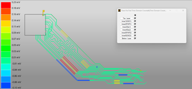
Figure 27: Crosstalk level along each trace
- Coupled Structures
From the crosstalk results, SIwave can predict the coupled sections. This means SIwave cannot treat the trace as a single line in the red sections. They look in SIwave as if they are coupled.
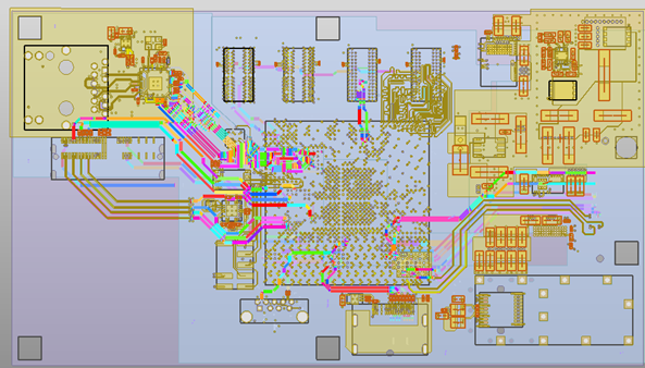
Figure 28: Coupling degrees in each section of all the traces
The designer can learn much about PCB grounding from the SYZ-solver, the Frequency domain, and the time domain analysis. If there are any issues, the user has the tool to zoom in on the weak areas and fix them.
