
SIwave is a power integrity and signals integrity tool. The signal net-analyzer solver is one of the tools in SIwave.
Signal Net Analyzer is part of the signal integrity bundle of SIwave. It does fast signal integrity calculations of the traces. It calculates the impedance, the delay, the loss, and many other things. It allows the user to study the effect of trace loss and any imperfections on an injected signal. Users can use pulse, PRBS, clock signals, and IBIS models.
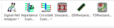
Figure 1: Signal Net Analyzer
SIwave should not be used to build PCBs. While this is possible, it is not the best way to utilize SIwave. But instead, try to import files from a professional CAD tool. SIwave can import the following type of CAD files:
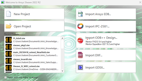
Figure 2: Import files
Any process in SIwave starts by selecting the solver. Once a solver is selected, a dialog box pops up, and all the user needs to do is to fill up the form and submit it.
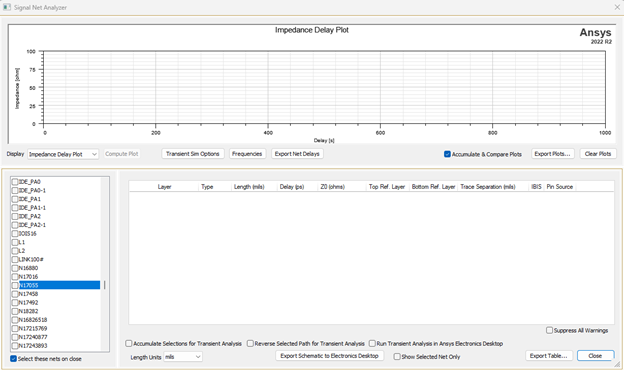
Figure 3: Signal Net Analyzer Dialog box
- Impedance Plot
The bottom left section lists all the powerplanes in red and all the traces in black. Select any of them, say the N17055, and SIwave automatically populates the bottom middle section with information about this trace. It displays the different sections of the trace, on which layer, the length, the delay, the impedance, and the reference ground on top and bottom. Select the name of the trace, and automatically SIwave plots the impedance along the path.
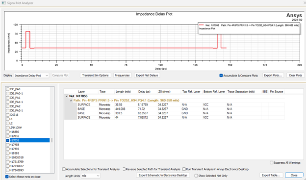
Figure 4: Impedance plot
The user can select another trace, like PB_WR#, and have the same information again. The two curves are plotted on the same graph because of the option: accumulate & compare plots. If this option is unchecked, SIwave will plot the last one selected alone.
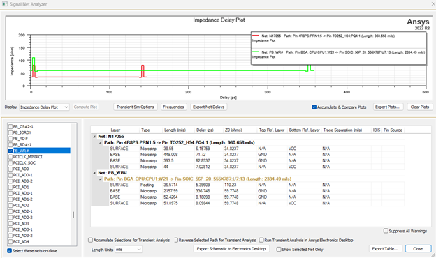
Figure 5: Impedance plot of many traces
One option in SIwave is to export the plots to an Excel file using the export plots. One can also export the net delay the nets to an HTML file using the export net delays. The result is an HTML file. The HTML file is an interactive page, so the user can post on a website and give access to colleagues to see the results.
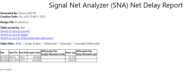
Figure 6: HTML files
Users can add markers, notes, and limit lines to the plot to be able to use it in any presentation.
Selecting a power plane will pop up a warning from SIwave because it was not made for powerplanes. Suppress these warnings by checking the box: suppress all warning messages. If the user wants to analyze a power plane, SIwave will create a set of data for every possible link between any two components attached to the board.
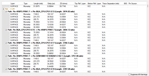
Figure 7: Power planes information
Same thing if the user selects a trace with no pins. A warning message will pop up. This is because a pin for SIwave is a port. If there are no pins, there are no ports on this trace.
Going back to the plots:
It shows the impedance along the path. This is not a TDR plot. The total delay is the actual delay of the trace. These plots are done at one specific frequency. This frequency is determined from the options. One needs to close the application first, then call the options to access the options. Close it first, then open the options.
- Signal Net Analyzer Option
In the option, we see the number of frequencies used in the calculations first. Select one, or select many of them. These will affect the transient response, which will be discussed later in this article. If many frequencies were selected, the user must select one of them to calculate the Zo impedance. Zo is always calculated at one frequency. Click on the set Range to enter the frequency range.
First, we will select one single frequency.
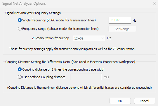
Figure 8: Signal Net Analyzer options
The solver uses the second section to determine if two traces are considered differential. It looks at the spacing between them. They are considered coupled if it is less than eight times the width or any custom value. The user can change that.
- Transient Analysis of the Traces
Back to the solver to do transient analysis. The transient solver requires a signal. The user needs to define the type of signal, then click on Managing Sources to enter the voltage, the impedance of the source, the rising/falling time, and the bit rate.
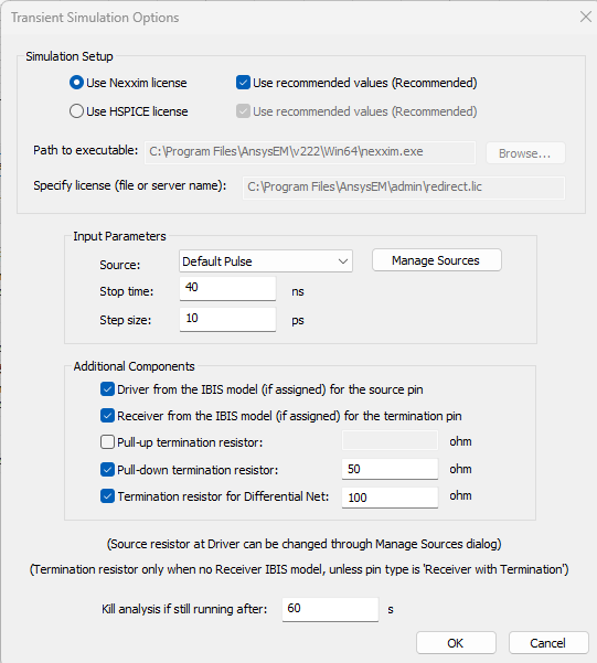
Figure 9: Transient solver options
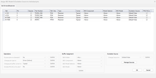
Figure 10: Modifying signal parameters
Select a trace, select transient, then compute the plot. And the results are plotted. The user can select to accumulate results by checking the box at the bottom: Accumulate selections for Transient Analysis.
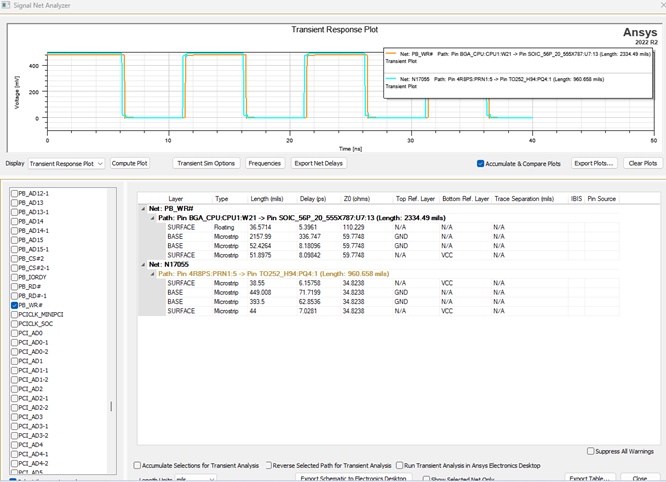
Figure 11: Transient results using single frequency option.
The user can also reverse the direction, i.e., excite the output with a pulse and watch the received signal at the input. Also can change the unit of the length inch to something else.
Repeat the transient solution and use a frequency range. Close the solver, go back to the options, and activate the multi-frequency one. Notice how the curve changes and becomes more realistic. That is why one needs to specify a frequency range for the transient solution.
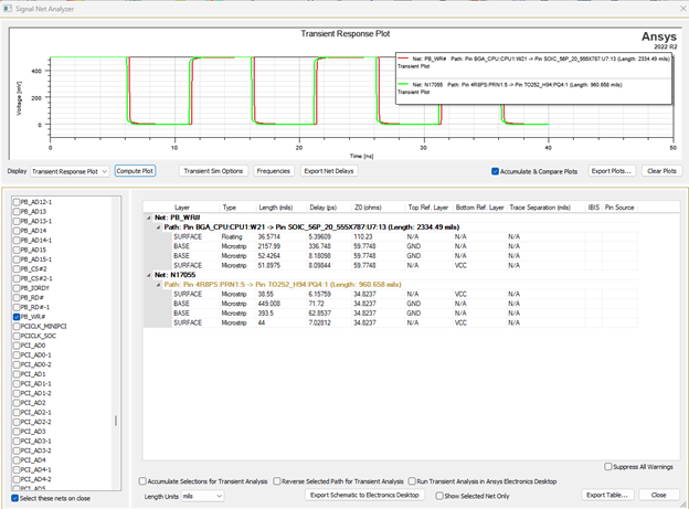
Figure 12: Transient results using a frequency range.
- Adding IBIS models
How to add IBIS models? This can be done from the model itself. Close the solver. Click on a component connected to an end of a trace, then right-click to get the small toolkit.
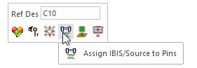
Figure 13: Component's small toolkit
Select the add-ibis button, and a new dialog box will open. Go to the pin of the trace. In this case, it is pin one and assigns an IBIS mode. All IBIS models are saved in a directory :
C:\Program Files\AnsysEM\v231\Win64\buflib\IBIS.
The list includes FBGA models like Cyclone and Virtex and RAM models like MT. If the user adds any file to the IBIS directory, it will appear in the list. SIwave uses a PULSE signal by default, but the user can select different signals on different pins. The change can be made in the same dialog box of the IBIS models.
Go back to the Signal net-analyzer to find these IBIS models and the Pins definitions in the table.
Figure 14: IBIS dialog box
- Export to AEDT Circuit Tool
The user can do more things with Ansys tools but needs to move all the analysis to the electronic desktop circuit tool. The circuit tool comes for free with SIwave. Click Export Schematic to Electronic Desktop, and SIwave will do everything. It will generate the schematic, including an eye source and probe. This will allow the user to do signal processing and even more which is Signal Integrity. Notice how SIwave represents the traces as a transmission line and the vias as an RCG circuit. No inductance in the vias.
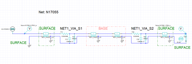
Figure 15: AEDT schematic
In the analysis of the AEDT circuit, just add the Verify eye to see the BER bathtub of the data and Quickeye to do eye analysis. They will be explained in another video related to signal integrity.
Signal net-analyzer can do the following calculations:
- Trace sections.
- Sections impedance.
- Sections locations.
- Sections delay.
- Transient solver.
- Use Pulse, PRBS, or clock signal.
- Use IBIS models.
- Export schematic to AEDT.
