
SIwave is a power integrity and signals integrity tool. In this article, we will be talking about the TDR (Time Domain Reflectometry) wizard and all its features.
TDR is necessary to examine the impedance of the traces in a PCB, detect any discontinuity, and identify issues with any transition, primarily via transitions. TDR is extracted from the s-parameters. Note: The user needs the Enterprise option to have access to the TDR wizard.
SIwave can do fast but accurate TDR calculations of hundreds of traces in large boards. No other software can beat SIwave.
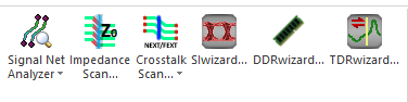
Figure 1: TDR Wizard
It is not recommended to use SIwave to build a PCB. Although one can do that, that is not the right way to use SIwave. SIwave can import the following type of CAD files:
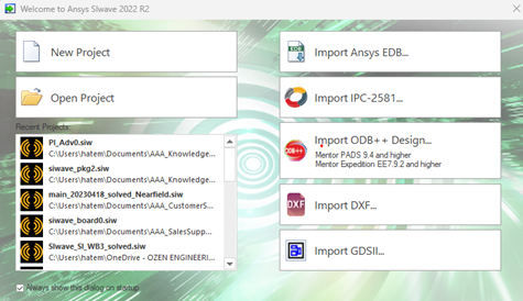
Figure 2: Import dialog box in SIwave
SIwave extracts lots of information from the CAD file, the stackup, the materials, the components, and the nets.
Select the TDRwizard from the solver list. Any process in SIwave, DC, PI, SI, or radiation starts by selecting a solver. Once a solver has been selected, SIwave generates a dialog box that looks like a form. The user needs to check the form and fill up the missing information. For example, the figure below shows the dialog box of the TDR solver.
To the left is a list of all the traces. Notice the tabs, single-ended, differential, extended, and extended differential. Select the traces you want to analyze by adding them to the right list.
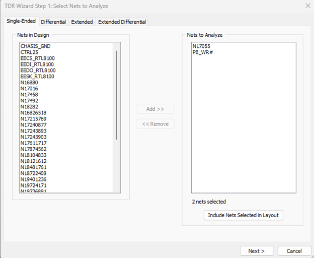
Figure 3: Select the traces
The next step is to specify the TDR probe location on each trace. Each trace must have one TDR probe and one termination. If the trace is a differential line, the user must select the positive and negative TDR probes and the positive and negative terminations.
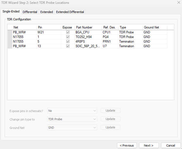
Figure 4: Add TDR probes and TDR terminations
The next step is about the specifications of the signal used in the TDR analysis. The user needs to specify the rising time, the pulse width, and the pulse period. Usually, the pulse width is set to a long time, longer than twice the trace's length. And the pulse period is set to double the pulse width. One can also set the delay. The user also has to confirm the values of the terminations.
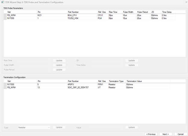
Figure 5: Add signals
The last step is the solver. The first section is the solution's name and what the user wants the TDR solver to do after solving it. After finishing the TDR solution, SIwave immediately transfers the data to the AEDT circuit. When it does that, it can create a schematic or just a netlist. But in both cases, it will display the TDR results. If the user selects the Use Ansys Electronics Desktop-SIwave Dynamic Link, SIwave will generate a full schematic in AEDT. The user can then use the schematic or modify it.
The second section is the step number and the stop time. Set it to one-fifth or one-tenth of the rising time of the signal. The stop time could be the pulse duration.
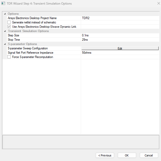
Figure 6: Add the solver
In the third section, click on Edit. Here you specify the frequency band. Notice that selecting the highest frequency will affect the minimum rising time the user can have. Trying different bands until the rising time matches the one specified for the signals.
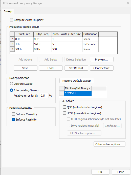
Figure 7: Specify the band and the accuracy of the solver
Press OK twice to start solving.
1. Ansys Electronic Desktop:After finishing solving the problem, SIwave creates a schematic in AEDT. The schematic has TDR probes and terminations. SIwave plots also the TDR impedance response and the voltage response. Since the schematic is available, now the user can do many signal integrity calculations. The box in the middle is just an s-parameters file.
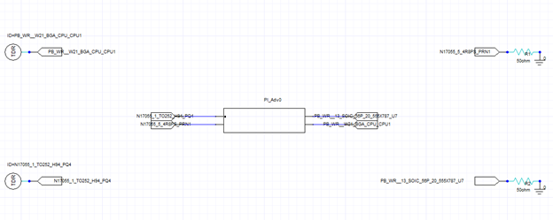
Figure 8: Schematic in Electronic Desktop
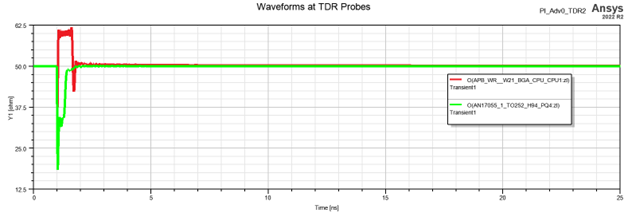
Figure 9: TDR plot
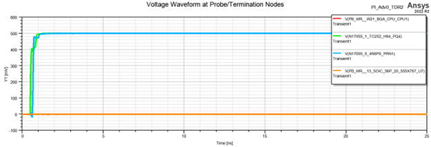
Figure 10: Voltage response
2. SIwave:As we mentioned, the TDR solver is just an SYZ solver. So it has all the S-parameters of the traces. Right-click on the solution, and one will see all the options of the SYZ solver. Another video about the PI solver explained all these options and their meaning. Notice that in SIwave, we can only process the s-parameters. There are no Signla integrity calculations in SIwave.
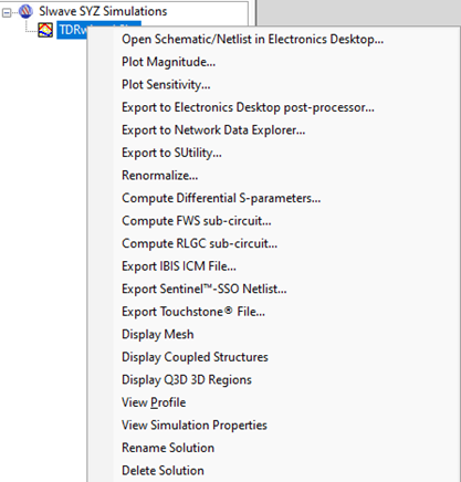
Figure 11: SIwave S-parameters options
3. SIwave:
To improve the accuracy, the user can use HFSS regions inside SIwave. The way to do that is to add a region extent. Go Home, then select one of these shapes in the Draw Geometry.
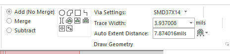
Figure 12: Adding extent regions
Draw a rectangle, for example, in a region in the PCB. Ensure that the boundaries of the rectangle cross the traces in straight clear sections. Avoid crossing transitions and vias.
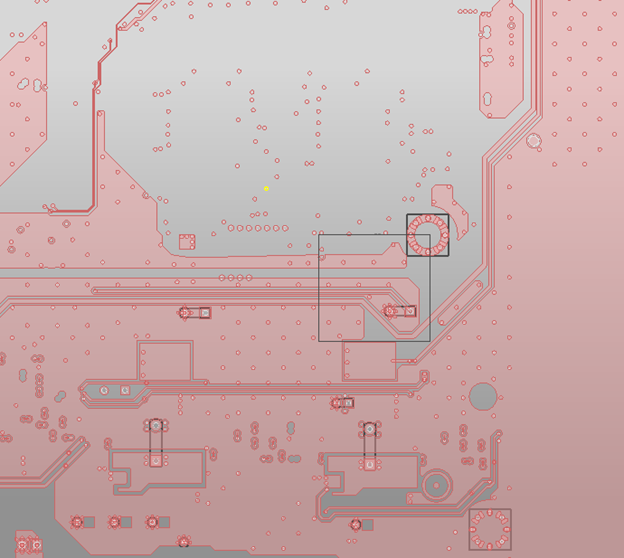
Figure 13: Select the HFSS extent region wisely
Then when setting up the solver, activate the HFSS option in the 3D solver.
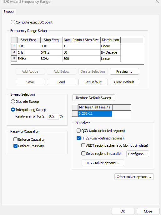
Figure 14: Activate the HFSS option in the solver setup.
