
SUMMARY
In structural analysis, there are two primary time integration schemes used to solve simulations. The Implicit scheme is employed in Static, Linear dynamics, and Transient analysis. In this case, the Newton-Raphson Method is utilized to solve each load increment, allowing for the use of larger time increments. The second scheme is crucial for short-term and highly nonlinear analyses, known as Explicit dynamics. This method is appealing because it does not require any iterative process and guarantees a solution for each timestep. However, it comes with a limitation on the time increment to ensure stable solutions, which is usually shorter compared to the time increments used in implicit analysis by several orders of magnitude.
Here, the user’s question is: What can I do when I need to solve a highly non-linear, long duration problem where inertia is not important? This scenario falls between the realms of Implicit and Explicit Analysis. It would be great to have the advantages of both in the same simulation. The solution lies within the concept of the 'Semi-Implicit Method,' as highlighted in this blog.
DETAILS:
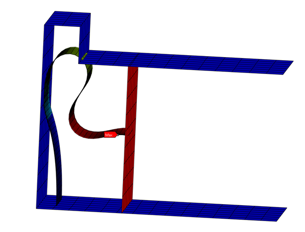
As an example, let’s consider a flexible band which must be enclosed in a fixed space while a wall moves rigidly reducing its volume. This band is attached at one end in the fixed side and the other at the mobile wall and is long enough to prevent stretching at zero displacement.
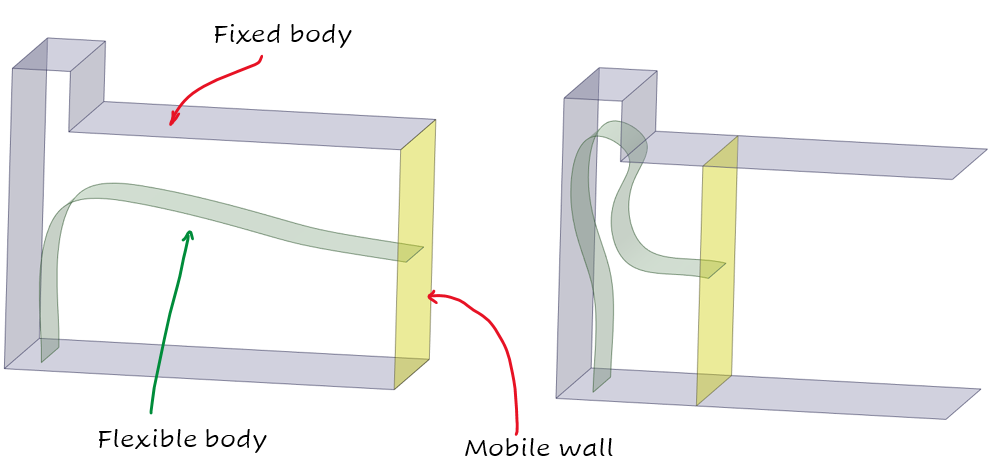
This model encounters highly nonlinear conditions, due to large displacements, rotations and sudden changes in contact status. We expect a relatively straightforward solution process initially, with increasing complexity towards the end, particularly at the point where the band 'snaps' into the upper chamber.
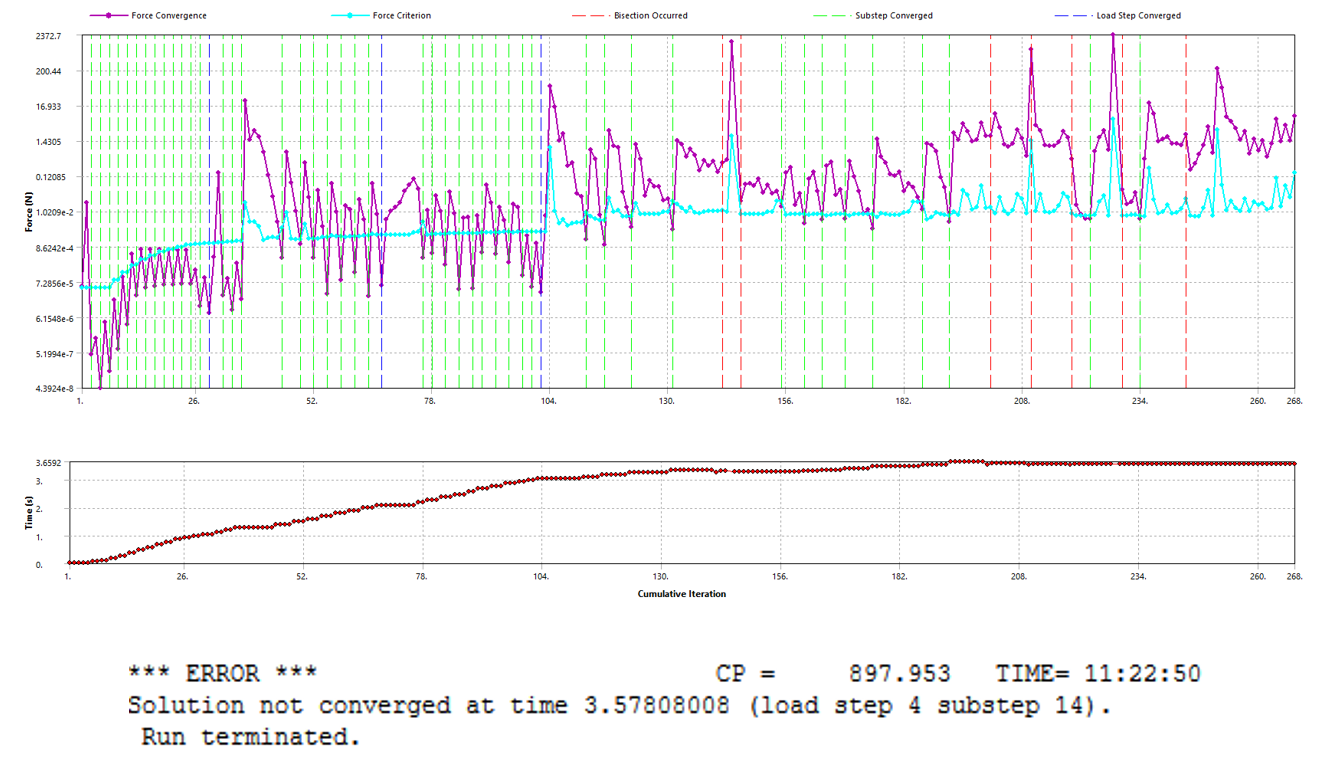
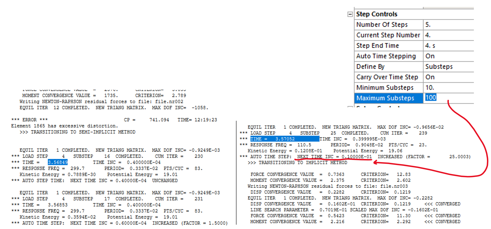
The total simulation time is 5 seconds. In the first three load steps, there are no convergence issues, thus few iterations are necessary, 104 in this example. Starting the fourth, the solver struggles with the solution until it stops at t=3.57 seconds due a convergence error. The increased number of substeps is noticeable here due to the initial contact and subsequent bisections. From iteration 201 onwards, successive bisections are employed to decrease the load step size in an attempt to achieve convergence. The last successful substep converges at iteration 234, following which the simulation ultimately fails at iteration 268.
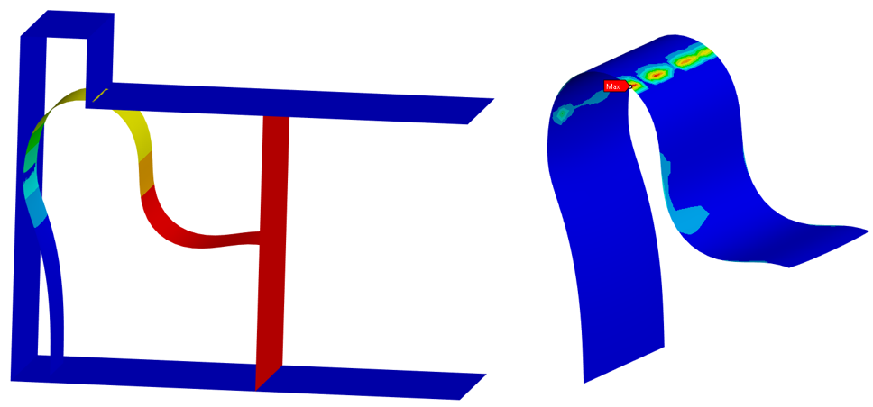
At 3.57 seconds the wall rigid displacement is not finished, and the upper contact is close to pass the corner as seen in the deformation contours. In the right, the residuals contour shows this zone as problematic.
USING THE SEMI-IMPLICIT METHOD
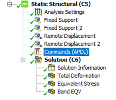
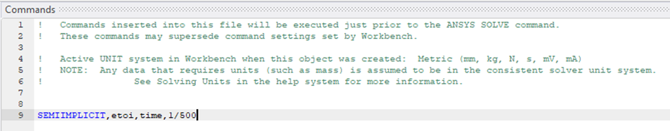
This method is designed to facilitate the passage the highly nonlinear short segments of the simulation before returning to the implicit phase. Here, an inertial force is calculated and subsequently added as a residual once the solver reverts to implicit. To implement this, the SEMIIMPLICIT command is utilized before SOLVE in the solution solver only for Static and full transient analysis types. In Ansys Mechanical it’s possible to include a Commands object to the analysis in the outline tree. It’s only possible to utilize this command in the first load step or after a restart.
The most popular option is ETOI, which indicates the amount of time spent in Semi-Implicit phase. Once this time is over, the solver returns to the implicit phase. For the example, the solver will solve 1/500th time units using Semi-Implicit before returning.
With this command, the simulation behaves like that:
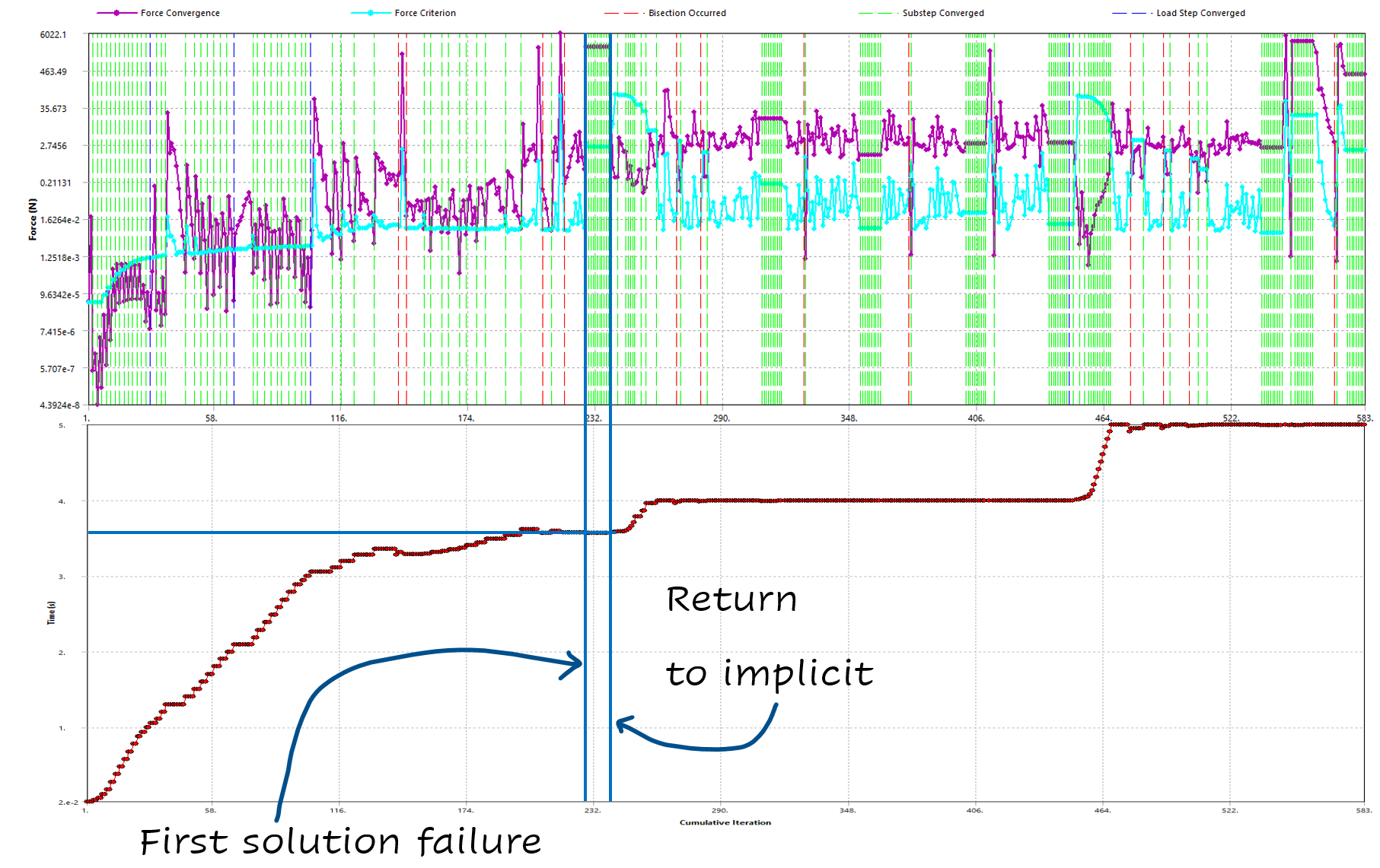
During the change to Semi-Implicit, in the solver output appears the message '>>> TRANSITIONING TO SEMI-IMPLICIT METHOD' at 3.568 seconds, then it returns at 3.568+(1/500)=3.570 s and uses the littlest time step defined in 'Analysis settings' for that load step.
Throughout the entire simulation, we can observe eight occurrences where the semi-implicit method is automatically activated each time the solver finds nonconvergence issues, all of this using the single line added in the Commands object. In the force convergence graph, these instances correspond to zones where the substep converges in one iteration, yet the residual exceeds the defined criterion. The total deformation looks better now and the imposed displacement is complete.
RECOMMENDATIONS
It is advisable to designate a short time for the semi-implicit phase. While the semi-implicit method aids in managing brief periods of extreme nonlinearities, transitioning back to the implicit solution can be computationally demanding. If the problem exhibits consistent extreme nonlinearities, it may be better to continue using the semi-implicit solution throughout.
All nodes in the model must have associated mass, requiring material density to be defined for at least one element.
When encountering issues during the semi-implicit solution with contact elements, reducing the contact stiffness and pinball value can aid in resolving spurious contact detection failures.
In problems involving contact elements, a high mass scaling can lead to large time increments and penetration, resulting in excessive contact forces. Adjusting the safety factor and mass scaling can alleviate these issues.
This method can be used in statical and full transient analysis types. Using transient Analysis may help with the transitions between stability states thanks to inertia and avoid some changes to semi-implicit.
CONCLUSIONS
This hybrid method is a advantageous way to use bigger timesteps in the implicit phase, when the non-linearities are not so strong to use Newton-Raphson approach. Once the non-linear model is too difficult to solve, the semi-implicit phase allows the use of explicit formulation to continue the analysis reducing the time step.
The Semi-implicit method is easy to configure, just a line in a command object makes it available in the simulation.