
SUMMARY
In this blog the Initial state technique which is used to create a non-zero stress or strain initial condition is presented, and a physical interpretation is shown. A simple example consisting of a beam and a thin layer of prestressed material is created using the INISTATE command to show the detailed steps.
INITIAL STATE
‘Initial state’ denotes the condition of a structure at the beginning of an analysis. It is commonly assumed that the structure starts in an undeformed and unstressed state, although this scenario may not always reflect real-world conditions accurately.
There are several applications for the initial stress (or strain) state. The most popular is adding thin layers of coating over existing substrates that develop stresses due to the manufacturing process. This is a typical procedure in the MEMS (Micro-Electro-Mechanical-Systems) industry. However, it is worth noting that this technique can also be employed in oil and gas structures where it is important to consider residual stresses from the welding process or initial deformations, among many other examples.
One common technique used to develop this state is using thermal conditions, even if they are not realistic. A nice Ozen video explaining all the process can be seen here:
The capability to account for the initial state enables the definition of a more complex starting condition for the analysis. For instance, it allows for the specification of an initial stress or strain state within the structure. In this blog we will explore this advanced analysis in Ansys Mechanical.
Form the physical interpretation to the finite element model:
Before going into the details of Initial state, let’s see an interpretation of the physical phenomena modeled and how it will be included in the numerical model.
Let’s consider an elastic band with no stresses or strains. Then, a force or displacement is applied to the band, increasing its length (while ignoring lateral shortening). At this point, we expect the band to experience tension stress as it becomes larger. Later, upon releasing the band, it will return to its original shape and reach a zero-stress state. This might seem like a trivial observation. However, consider what happens from the moment of release to the final state. The band seeks an equilibrium state, and with no constraints, its only option is to return to its original shape, releasing all the applied stress through external displacement.
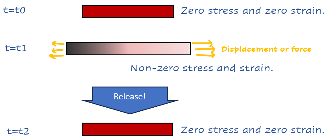
At this point, we can consider these three time steps according to the finite element modeling process. We can designate the instant t1 as the 'initial state,' wherein there exists a deformed geometry and developed stresses. The moment t0 is not significant and will not be included in the analysis because we lack knowledge regarding the stress origin, and there is no interest in calculating it. Finally, at moment t2, the stress solution is computed between t1 and t2 by solving equilibrium conditions for this body.
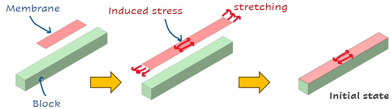
Is possible to define any kind of objects in the simulation at t2, this is the actual simulation interest. Now, let’s consider the same elastic membrane and a block which is larger than the membrane. When the membrane is stretched to match the length of the block, longitudinal stresses will develop. Finally, after bonding these two bodies, we have the initial state, and this is how the finite element model will be created letting behind the previous stages.
USING INITIAL STRESS
This method is designed to by applied using the INISTATE command. The process is presented using the previously defined example.
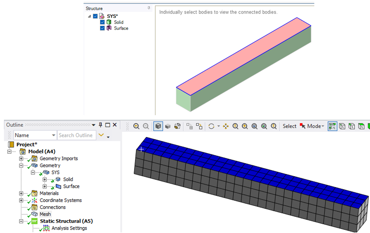
- Geometry and mesh:
Remember, the initial stressed geometry must be represented as the deformed shape, as mentioned before. Just a block and a shell are enough for this. To facilitate interaction avoiding contact elements between bodies, ‘Shared topology’ was defined in SpaceClaim, which allows the shell and the block to share nodes. Default meshing in this geometry will generate hexahedral elements.
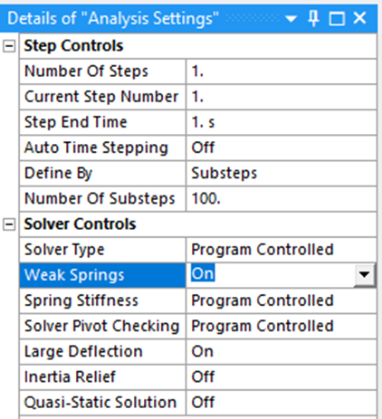
- Boundary conditions and solver settings:
In this example there are not boundary conditions defined, that depends completely on each model. To avoid rigid body motion and convergence issues, ‘Weak Springs’ property is defined as ‘On’. ‘Large deflection’ is activated too and 100 substeps lets follow the solution using intermediate results.
- Inistate command:
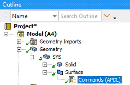
This feature is not available directly on the Mechanical interface, that is why we need to include APDL snippets in two sections of the model tree.
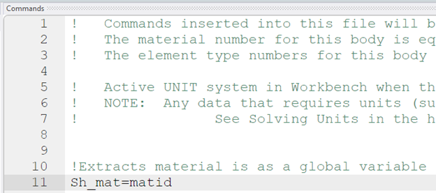
The first one is inserted on the body to be affected by the initial stress, in this case, the surface. Here just a variable is defined to extract the material unique number for this particular body. This will be used in the next section.
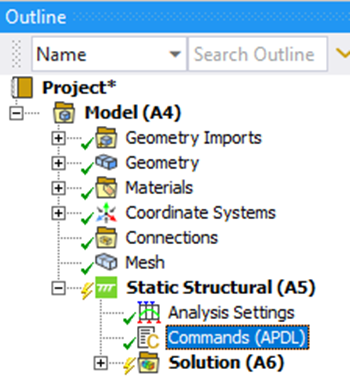
The second snipped is added to the analysis under ‘Static Structural’ branch. This will make these added commands be executed just before the solving process.
The command lines are the following:
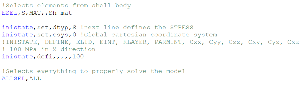
ESEL selects the shell elements using the Sh_mat variable created before. This is a generic way to select the appropriate elements, this can be done in several different ways.
The INISTATE command is executed three times to define the use of stress as initial value, then to especify the global coordinate system as direction for the stresses applied and finally to assign the value of 100 MPa (that depends on your solver units) in element local X direction, this is the Cxx parameter for the command. To define stresses in additional directions, we would use Cyy, Czz, Cxy, Cyz and Cxz arguments.
Finally, the ALLSELL command allows to select everything in the model before solving. Forgetting this last line may generate errors during the solving phase.
Warning: Coordinate system.
If you look into the .out file, a warning message is displayed referring to shell coordinate system.
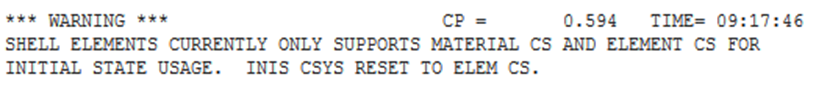
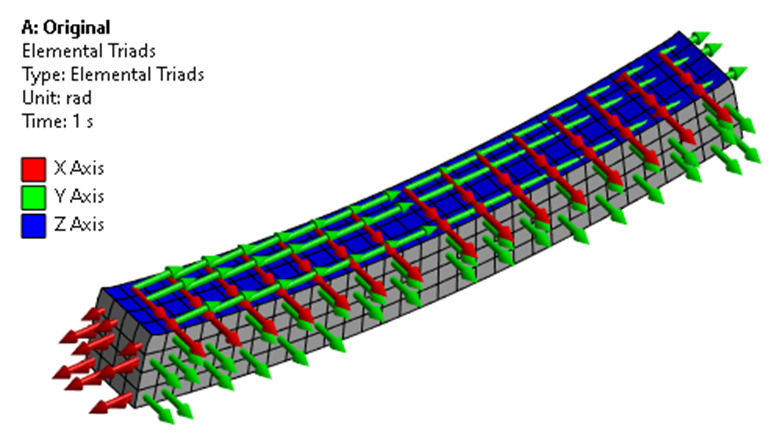
The global coordinate system is established in the second line using the INISTATE, SET, CSYS, 0 command. However, shell elements do not support initial states in the global coordinate system. Consequently, this definition is reset to the element coordinates, which is equivalent to using INISTATE, SET, CSYS, -2. Therefore, users must ensure the correct definition of stress direction. In this example, the shell element's X direction (depicted in red) is perpendicular to the beam’s longitudinal direction. Hence, the correct stress direction should be Y and defined with the Cyy argument.
The corrected script should be:
ESEL,S,MAT,,Sh_mat
INISTATE,SET,DTYP,S
INISTATE,SET,CSYS,-2
INISTATE,DEFI,,,,,,100
ALLSEL,ALL
- Results:
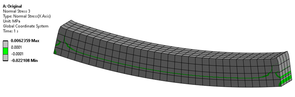
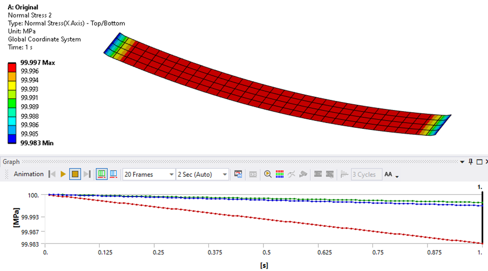
After solving the model, it is evident that the block has developed some bending stress at the final equilibrium state. Note that the neutral axis is not located at the section’s centroid.
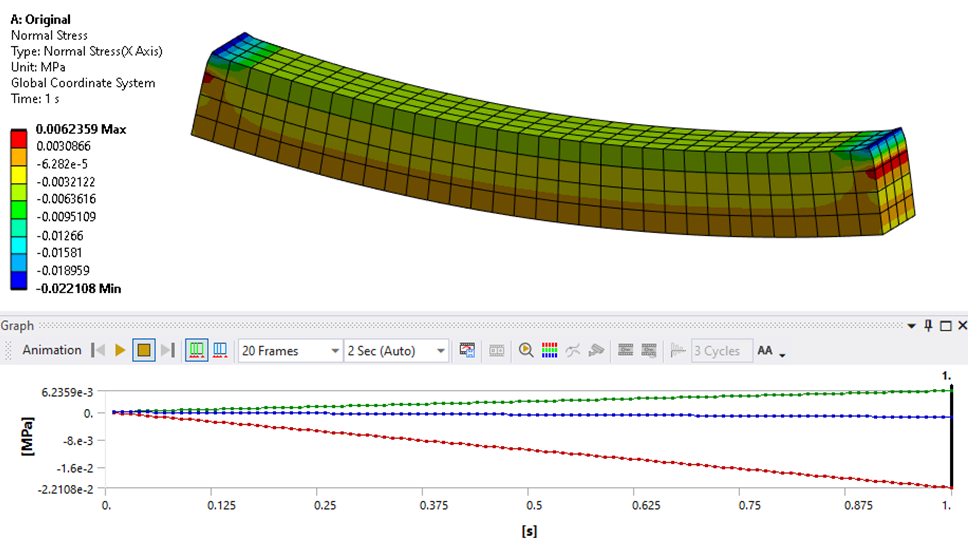
The stress in the shell is slightly reduced from its initial value of 100 MPa.
ADDITIONAL COMMENTS
INISTATE is a command with several options. You can use this command to designate the initial state coordinate system, data type (such as stress, strain, plastic strain, creep strain, among others). It is also possible to define the data on elements, nodes, layers, or Gauss integration points. Additionally, it can be used to export a solved stress state and to import data from existing data files. For further exploration, you can refer to the Ansys help documentation.
CONCLUSIONS
This command is useful for specifying an initial stress or strain state, enabling users to enhance analysis capabilities by considering more realistic scenarios without needing to solve the entire load history to obtain it.
The most complicated issue here is understanding its physical meaning and, consequently, its application. The advice here is to consider the search for equilibrium, as this is what the solver will do.