
TLDR: Ray paths are complicated. It has been challenging for designers to predict the performance of their design without a prototype. ANSYS HFSS can help designers predicting the radiation pattern in a real-world environment during the design process.
In the past, I have talked to a team of engineers who design GPS systems. They weren’t worried about antenna matching, because for off-the-shelf components it can usually be done by the manufacturers. On the other hand, they were quite interested in seeing the antenna radiation pattern.
Antenna design can be simple; but integrating the design into a system is often more challenging. Antennas in a circuit can be either receivers or transmitters. Engineers are often interested in the gain and directivity of the antenna. Here, I will discuss radiation patterns, power gain, and power dissipation of a GPS design.
Overview
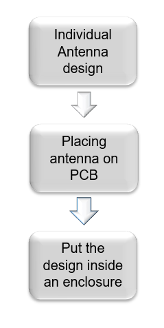
When talking about the performance of an antenna design, we all know that the antenna is normally designed under ideal conditions with ideal performance. However, in the real world, antenna performance can be impacted by its surroundings.
For example, if you are designing a GPS system, when you place an antenna on the PCB, does the result meet your expectations?
What happens if you put it inside a structure or enclosure?
What happens if you include an even larger structure? Do you still see a good result?
Topics covered in this blog
ANSYS has developed an easy-to-use tool for us – HFSS. HFSS is a 3D electromagnetic simulation software for high-frequency electronics.
If you think simulation is too complicated, I will show you that it’s much easier than you think. Plus, it can save you time and money during the design and testing process.
Example
Here, we have a GPS design for the demonstration.
I will show you how it behaves in free space, and when it’s placed inside a car model.
If you are interested in seeing the antenna behavior by itself, you can refer to the specification:
https://www.digikey.com/en/datasheets/johansontechnologyinc/johanson-technology-inc-1575at43a0040
Lastly, I will show the power dissipation on different geometry (lossy components).
Import
HFSS supports many different import methods. Typical file types include:
AutoCAD, ODB++, Cadence APD/Allegro/SIP, GERBER, ICP2581, AWR, etc.
If your file type is not any of the above, there are always more options in HFSS.
Design Setup
After your design is imported, make sure to check your model
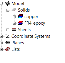
Model Detail
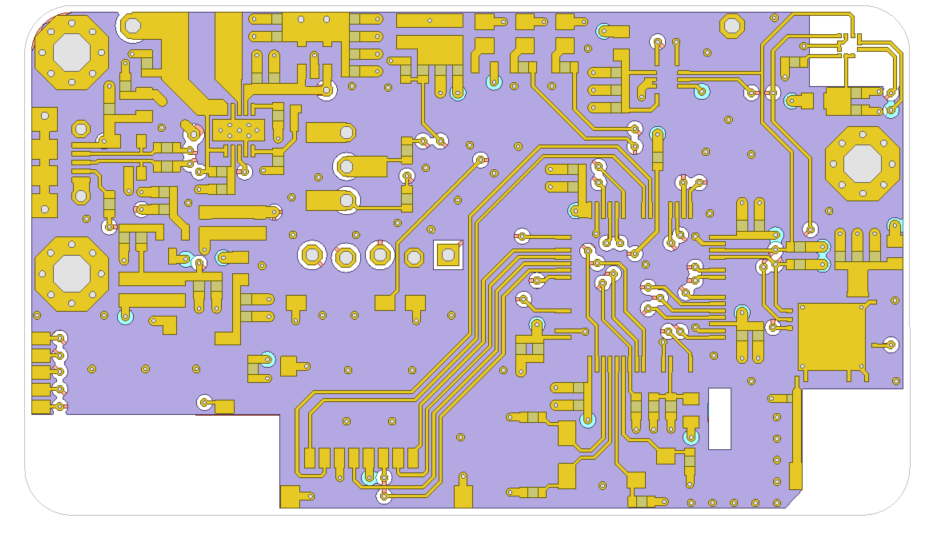
Board imported
If your antenna is from a manufacturer, it will not be imported. But you can always import it separately, either from ANSYS component library or an external 3D model.
The ANSYS component library includes many different types of antennas, and antennas from manufacturers such as TDK and Johanson Technology.
Or, you can import the 3D model if it’s not in the component library.
BOOM!
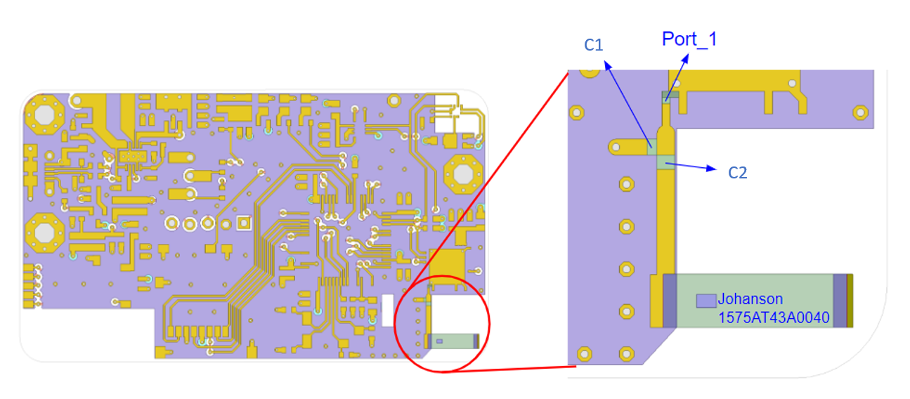
Completed design with antenna and matching components
By using drag-and-drop method, I placed the antenna at the proper position. In the picture above, you can see that some antenna matching is done.
A 50Ω port is set up and assigned excitation for simulation purpose.
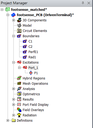
Project manager
Inside the project manager windows, you can check for the excitations and boundaries.
In HFSS, an airbox is required. And the size of the airbox is often time ¼ of the wavelength λ. For this design, the frequency of a GPS antenna is 1.575GHz. And 1/λ will be around 50mm.
You can create an airbox with absolute offset of the design using “create region”.
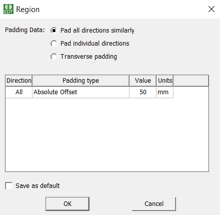
Create region
A radiation boundary is required to extract radiation pattern, and assigned to the airbox.
Or, on the schematic, right click à Create Open Region à Enter operating frequency & boundary condition.
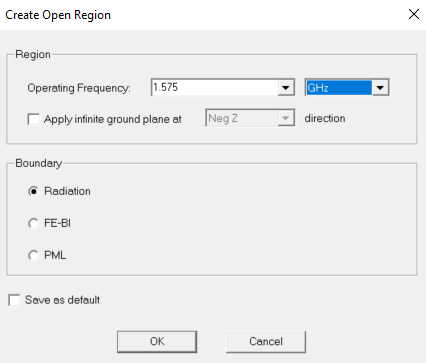
Create Open Region
The model set up is basically done at this point.
Few more things to setup the simulation: analysis setup and sweeping range.
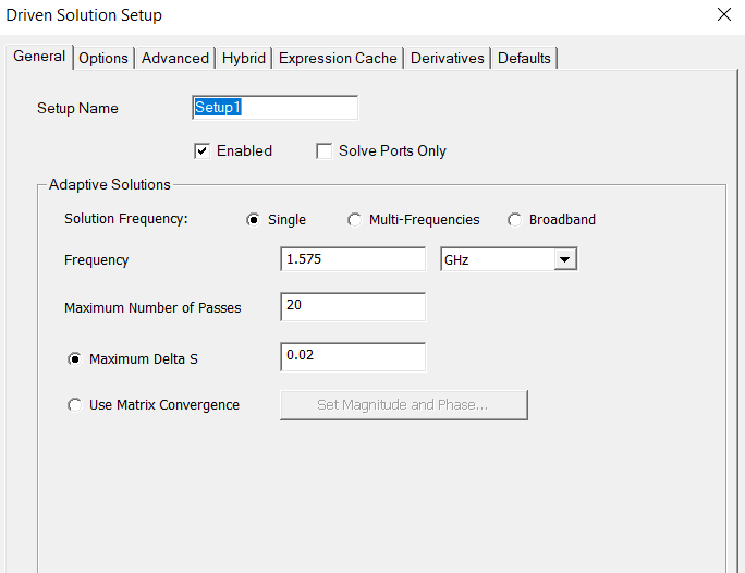
Analysis Setup
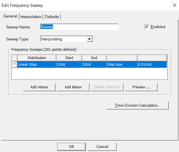
Sweep setup
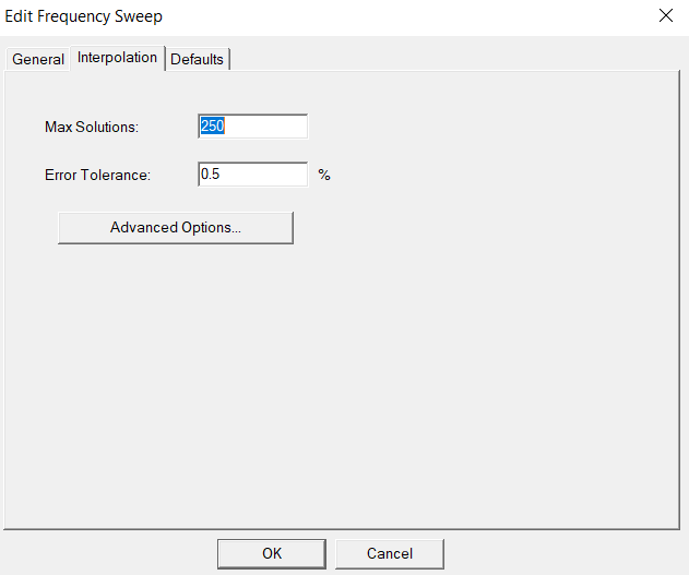
Sweep setup
You can choose the sweep type and range in this setting. As well as setting up the error tolerance. Different setting can affect the simulation time.
Setup is done, Simulation will be fun
The simulation time of this complex model can take over two hours to solve. Again, this can vary by the analysis setting.
After the simulation is done, Let’s check out the azimuth and elevation of the radiation pattern.
Go to project manager —> Result —> Far filed plot —> Radiation Pattern.
<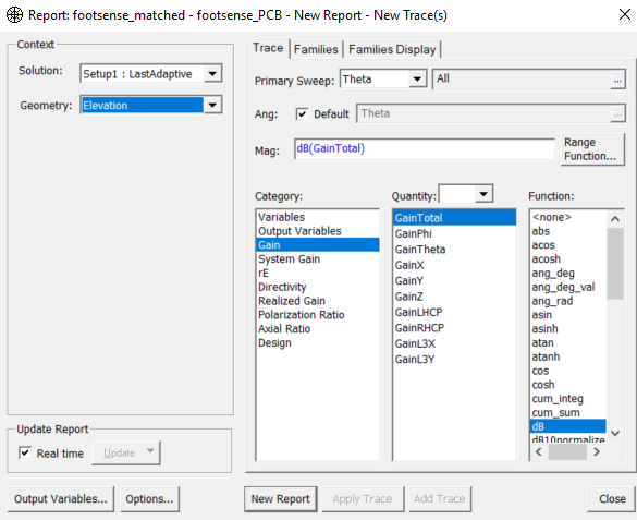
Create Radiation pattern
If you are interested in the 3D plot, then plot 3D polar plot in “Far field plot” instead of radiation pattern.
MAGIC!
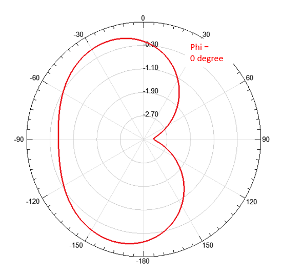
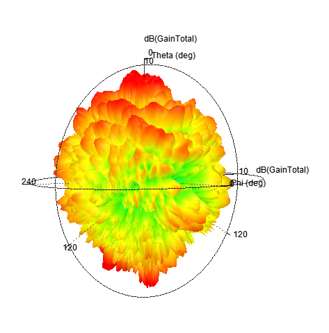
Here is your radiation pattern.
 <div
<div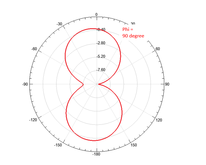
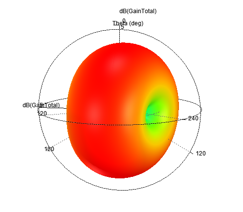
Antenna radiation pattern
This does not make sense? Check this out.
 <div
<div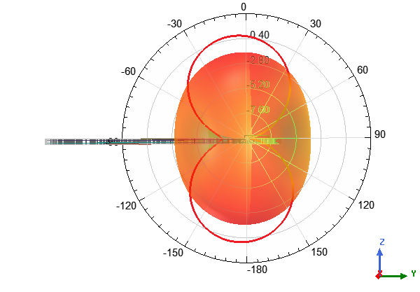 <div
<div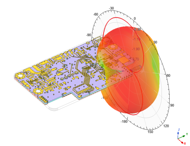
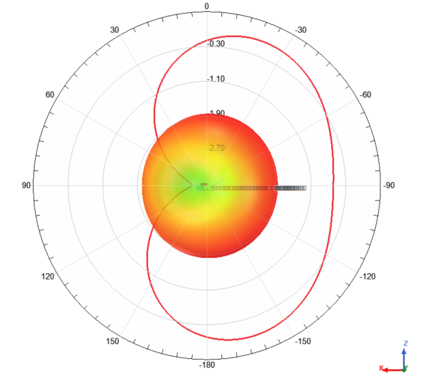
Radiation pattern on board
We are plotting the radiation pattern overlap with the design. This can provide you a better view of the antenna behavior.
Place it in a car
Now, we need a car… ANSYS allows to import any CAD model.
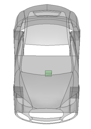
Car Model
The GPS design is placed in the front of the car.
Before running the simulation, we need to make sure the car is assigned SBR+ region.
SBR stands for Shooting and Bouncing Rays, it allows you to analyze the radiation pattern based on the number of ray bounces.
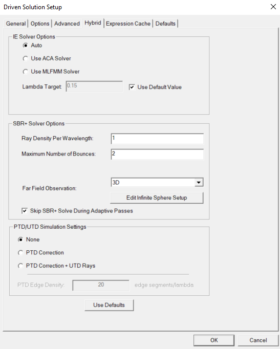
Hybrid Setup
In the analysis setup —> Hybrid tap —> SBR+ solver option, you can set the ray density and number of bounces. Increasing ray density and bounces will increase memory usage and simulation time. But accuracy will also increase proportionally.
Now, let’s check out our result.
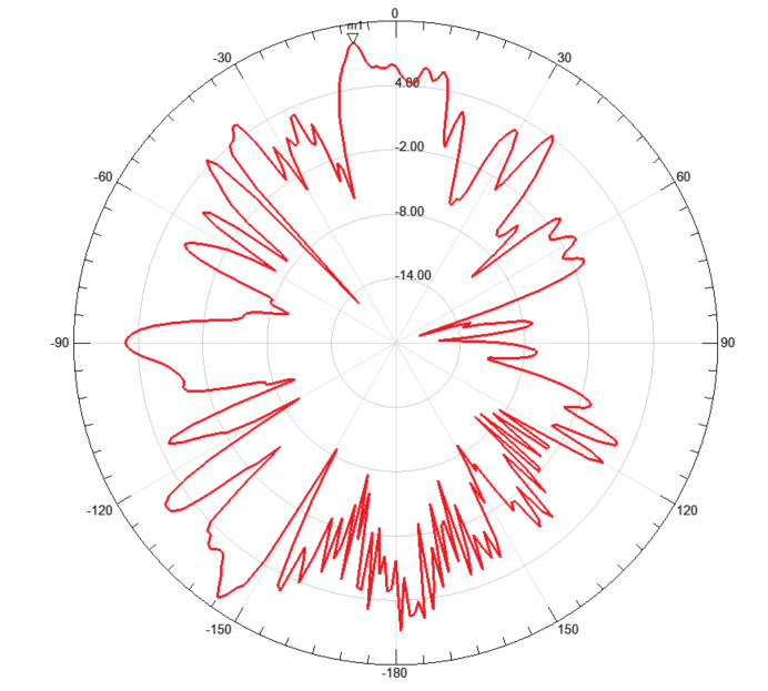
In Car Radiation Pattern
In Car Radiation Pattern
If we plot it over the model…
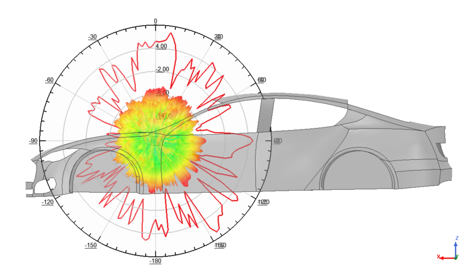
Radiation pattern with car model
As you can tell, the antenna performance can be impacted by the surrounding significantly.
What happen if we include the radome in the design and place in a different structure?
Power dissipation calculation
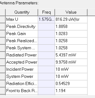
Antenna parameter
The radiated power of the antenna is ~5.44mW, which is only 54.5% of radiation efficiency. What happens to the other half of power?
HFSS allows you to calculate power loss in different geometry.
For example, what is the power loss in dielectric material with loss tangent of 0.02? Approximately 1.76mW
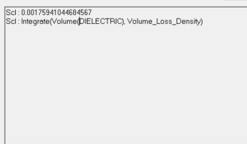
Dielectric power loss
We also have various model set up for further simulation, such as installed car radar performance simulation on the road.
Please contact us if you are interested or having questions.