
Basis of RMS Wavefront Error
In optical system design, abbreviation is critical to evaluate performance of the system in terms of image quality. Most used metrics to evaluate image qualities are mostly based on MTF and aberration plots. When translating aberration into a numerical specification, multiple methods can be complementary in different applications. In a telescope system with source as form of a point, for instance, Root mean square (RMS) wavefront error is a better option for image quality evaluation.
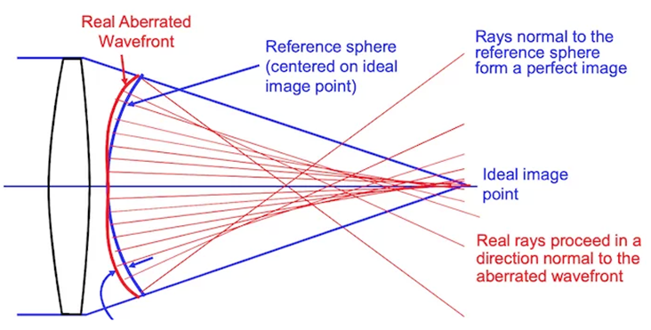
Figure 1 Wavefront error illustration
RMS wavefront error is to measure wavefront aberration. While spherical wavefront is for perfect case, most real light wave present various shapes to present potential image characteristics. Complicated description of wavefront description can be found in textbooks, which we won’t cover in this article. A direct comparison of morphological characteristics can be found in the upper figure. In concept, the RMS wavefront error is calculated as a square root of the difference between the average of squared wavefront deviations minus the square of average wavefront deviation. Basically, the RMS value expresses statistical deviation from the perfect reference sphere, averaged over the entire wavefront. It is a comprehensive measure of aberration in view of light as electromagnetic wave.
As shown in Figure 1 of demonstration of wavefront error, the reference sphere is centered on the expected image location, which is usually the image surface location of the chief ray. A different reference sphere will fit the actual wavefront. If the center of the better reference sphere is at a different axial location than the expected image location, there is a focus error in the wavefront. If the center of the better reference sphere is at a different lateral location than the expected image location, there is a tilt error in the wavefront.
RMS Wavefront Error Evaluation in Zemax of a Double Gaussian Lens
This lens is designed with 28 (±14) degrees of field, as shown in Figure 2 below. Design covered wave bands are in visible range (400 nm - 700 nm). While geometric MTF are calculated in 20lp/mm, all MTF values are higher than 0.65 (Figure 3). Spot diagrams in all three sampled fields and sampled wavelengths are shown in Figure 4.
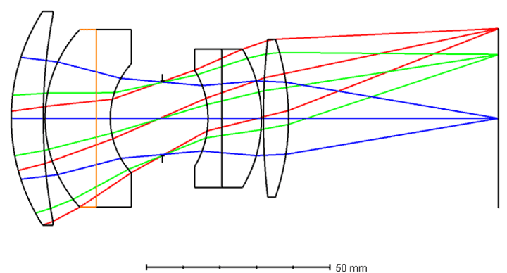
Figure 2 Layout of the lens
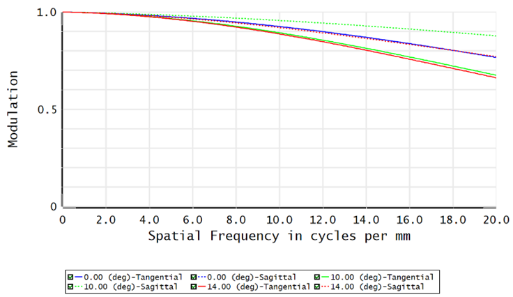
Figure 3 Geometric MTF up 20 lp/mm
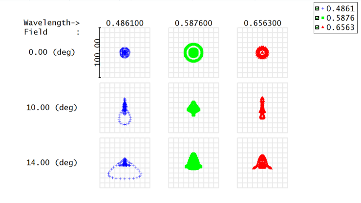
Figure 4 Spot diagram
Ansys Zemax OpticStudio reports wavefront errors at the Exit Pupil of a system. The errors are the difference between the actual wavefront and the ideal spherical wavefront converging on the image point. In a system with aberrations, rays from different positions in the exit pupil may miss the ideal image position by various amounts when they reach the image plane. Zemax uses a geometric relationship between ray errors and wavefront errors to calculate the wavefront error map. Since rays are always perpendicular to wavefronts, a wavefront tilt error corresponds directly to a transverse ray error (TRA) at the image plane. By tracing rays through the pupil, and measuring the TRA of each, we can get the slope of σ; then by numerical integration, we can find the wavefront aberrations, σ.
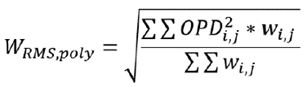
For RMS wavefront computations, OpticStudio always subtracts out a reference sphere. RMS wavefront error with the mean subtracted is computed as follows. where Wn is the optical path difference (OPD) at a given point in the pupil and Wn is the weighting at that point in the pupil.

If a polychromatic computation is done, the RMS polychromatic is done for all wavelengths at the same time and for all the pupil. The RMS polychromatic is computed as follows. OPDi,j is the Optical Path Difference of each ray at each wavelength. The OPD value will be a different value depending on the Reference (Centroid, Chief Ray). Wi,j is the weight of each ray at each wavelength. i is the indexing of the field and pupil position of each ray. j is the indexing of the wavelength used to trace each ray.
Figures 5-7 are RMS wavefront error as a function of field, wavelength and focus range of the lens in Figure 2. A perceptual observation can be obtained with these figures that the most wavefront error happens at a certain filed in Figure 5 (colors indicate wavelength) and wavelength in Figure 6 (colors indicate wavelength). Figure 7 illustrates wavefront errors in a tight focus depth.
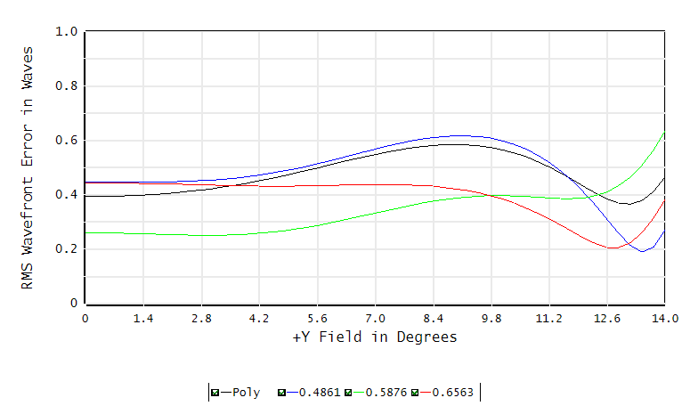
Figure 5 RMS wavefront error vs field, color indicates wavelength
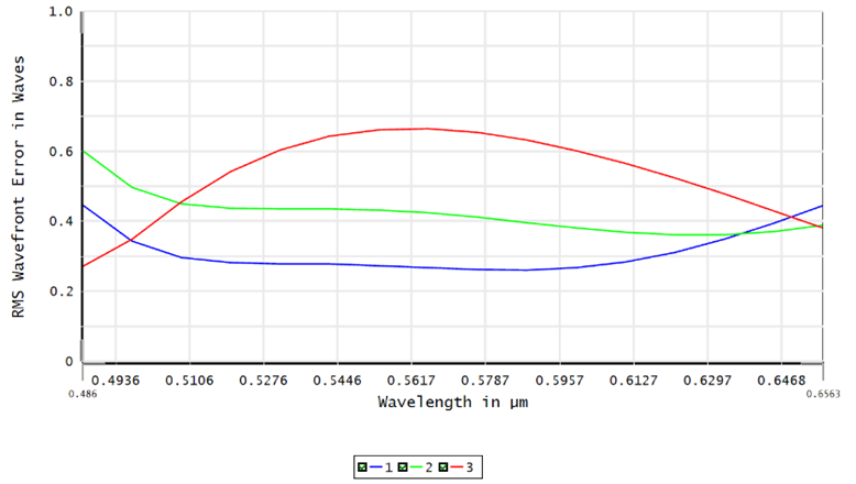
Figure 6 RMS wavefront error vs wavelength, color indicates field
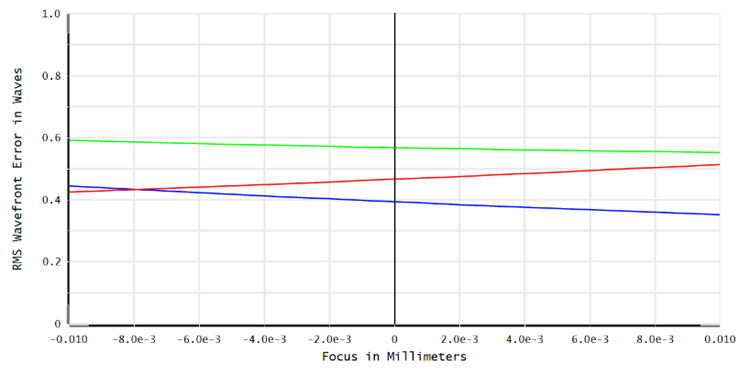
Figure 7 RMS wavefront error vs focus range, color indicates field
