
Summary
In the first part of this discussion series, I explore and verify the relationship between hand calculations and the time-dependent response of a object being dropped on to a rigid surface and what deflections and stresses occur during that impact period. The concepts discussed below are imperative towards understanding how to setup and solve a transient structural analysis using ANSYS Mechanical.
Figure 1: Bar during impact (with exaggerated deflection scale).
Figures 1 illustrates our example bar after being dropped and displays what happens during the period of impact. The remaining body of document explores how we can setup and analyze this type of system and compare our progress with common hand calculations.
Here is a list of topics which are covered in this discussion (in order of appearance):
- Potential Energy
- Elastic Energy
- Directional Stiffness
- Static Structural Analysis
- Average Compressive Force
- Kinetic Energy
- Impact Velocity
- Impact Period
- Natural Frequency
- Modal Effective Mass
- Transient Structural Analysis
- Analysis Duration
- Time-Step Frequency
- Complex Transient Displacement and Stress Results
- Average Compressive Stress
Details
I began to explore the relationship between hand calculations and maximum deflection and stress results produced by dynamic events, such as one object impacting another. I used ANSYS Mechanical as a means to verify assumptions and to provide greater details into these dynamic events. I have faith in the finite element method and I look forward to sharing my findings with you.
I started my exploration with a simple example of a cylindrical bar being dropped on to a rigid surface. In this scenario, and all scenarios associated with this discussion, I assume there is elastic material behavior and that none of the loads would cause plasticity or damage. This means that there is conservation of energy within the geometry.
During this process, I made a series of assumptions, performed finite element analyses to either verify, or dispute those assumptions. This process caused me to ask more questions, analyze, and get more answers. In the end, I am able to confidently describe many aspects of this dynamic event, all of which I will present as concisely as possible.
Let’s start with the simplest idea.
This first example explores the drop of a cylindrical bar on to a hard surface. The bar has a diameter of 25.4 mm and a length of 254 mm and mass density of 7.85e-06 [kg/mm³]. This bar will be dropped from 1 meter from the bottom face.
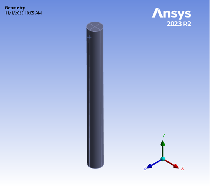
Figure 2: Cylindrical Bar
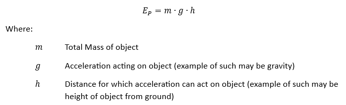
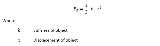
Under this circumstance, the potential energy must equal the elastic energy.
Potential Energy:
Elastic Energy:
Let’s equate our Potential Energy of our falling cylinder with its Elastic Energy to learn if we can predict deflections accurately.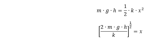
Let’s assume that the bar will be dropped such that it would travel in the negative Y-direction. Therefore, the first step will be to determine the stiffness of our geometry in the Y-Direction.
For our model, this stiffness can be derived theoretically, as well as by using the finite element method of applying a known load and dividing this load by the calculated Y-direction deflection. This will allow us to compare the results of our finite element estimation to the theoretically derived value and develop confidence in our methodology.
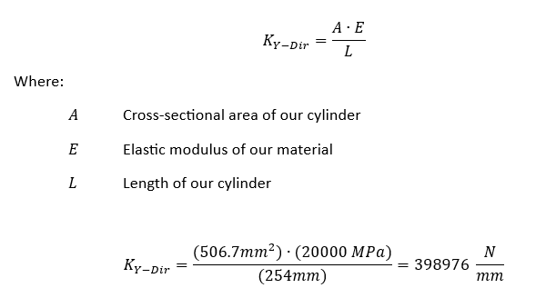
Let’s derive our theoretical stiffness. For the Y-direction, the following formula will apply:
Now, let’s also calculate the geometry stiffness through a finite element analysis by two different methods, so that we understand the different considerations involved with different types of loads.
Here we consider a fixed base while applying a force to the distal end of our cylinder such that the reaction force at the base is equal in magnitude and opposite in sign to the applied force on top of the cylinder. The magnitude of this compressive load is not critical, as long as our material properties are linear and that we are not considering geometry non-linearity (Large Deformation).
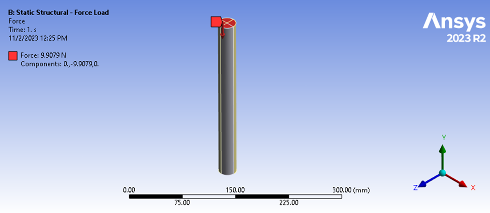
Figure 3: Static Structural Analysis of the rod loaded from its top and supported at its bottom.
In this scenario, a 9.9079 N load is applied to the top surface while the bottom surface is fixed from Y-displacements. The magnitude of this load will become more clear later.
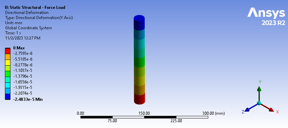
Figure 4: Static Structural Deflection Results
Solving the static structural analysis shows a maximum magnitude for our compressive deflection to be 2.4833e-5 mm. Based on our 9.9079 N load, we can calculate the following average stiffness.
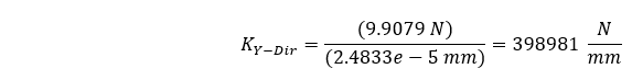
One can see that the finite element approach demonstrates only 0.00125% difference with the theoretical approach. This makes us feel good 😊
Next, let’s consider a different type of loading, such as gravity loading. Here, the force is removed from the top surface, but the bottom surface remains constrained, and gravity is applied at 9806.6 mm/sec^2. The reaction force at the base is 9.9079 N, but the force acting on the top surface is most definitely zero. The deflection results show a different deflection magnitude of 1.2421e-5 mm.
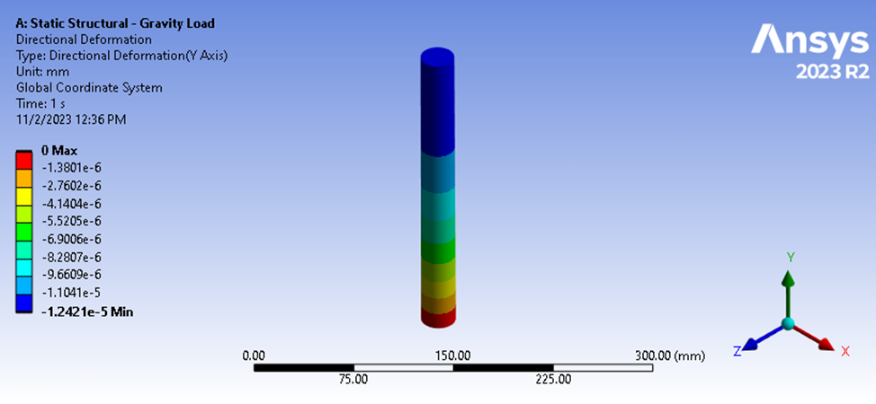
Figure 5: Static Structural Analysis Deflection Results
If we tried to calculate the stiffness by the same form of the equation as above, we would arrive at the incorrect value because we would not be considering the average compressive force acting though our geometry. In this case, our average compressive force can be estimated easily since our geometry has a constant cross-section and our estimated average stiffness can be calculated as follows.
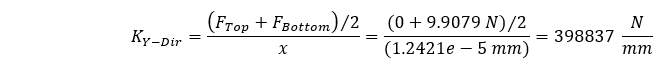
This estimation demonstrates a 0.0348% difference from our theoretically calculated value. Therefore, by two different loading methods, we can confidently estimate geometry direction stiffness.
Substituting our estimated directional stiffness, along with our model and material properties, we can estimate our maximum deflection below.
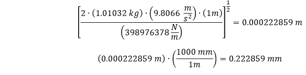
Which is around ~0.223 mm. Now we need a transient structural model to simulate the deflections at and after the time of impact of our cylindrical bar with the ground.
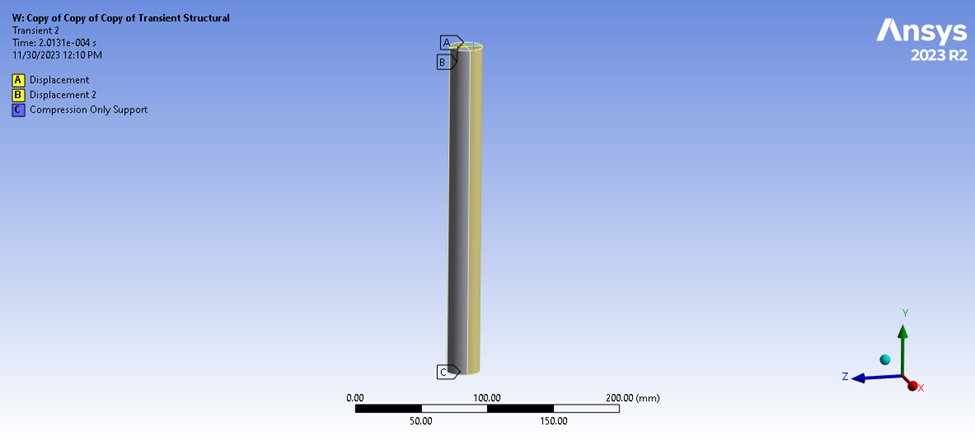
Figure 6: Transient Structural Analysis Model and Constraints
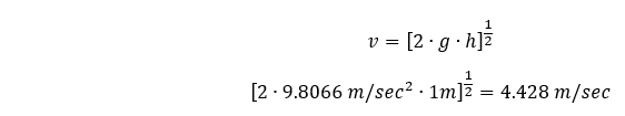
Our model assumes the bar is moving at 4428 mm/sec in the negative Y-Direction. This is the speed this bar would achieve if dropped 1 m. We can calculate this by equating the Potential Energy of the shaft with its Kinetic Energy at the instant of impact.
Kinetic Energy:
Therefore:
Constraints are added to maintain the vertical stature of the geometry, while a compression-only support is added to the base. The analysis duration is defined (more on this later), along with a frequent capture rate for gathering results.
The analysis results are complicated, because as the top of the bar is deflecting downward after impact, the bottom of the bar might be slightly compressed due to the stiffness associated with the compression only support. It is the difference in deflection between these two surfaces that describes the overall compression of the bar.
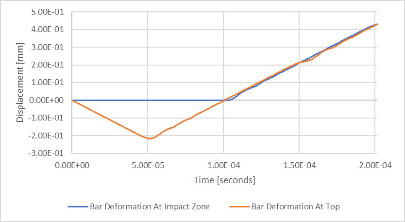
Figure 7: Transient Structural Deflection Results
The flat period of the blue line, “Bar Deformation at Impact Zone”, demonstrates that period for which contact at the base occurs, or the dwell associated with the impact. If we re-plot our data to focus on this period, we can more easily make several observations.
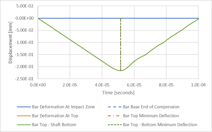
Figure 8: Transient Structural Compressive Deflection Results
I’ve added a green line which represents the difference between the bar top and bottom surface deflections, resulting in the total compression of the bar as a function of time. The two vertical dashed lines represent the time intervals associated with minimum results for orange and green lines. One may see that the minimum compression of the bar occurs at the same time as the minimum compression of the top of the bar. From this, we can estimate the maximum compression of our bar to be 0.216 mm, which is just under 3% smaller than our estimated maximum deflection of 0.223 mm.
There is, however, more to explore and learn from this example and its results.
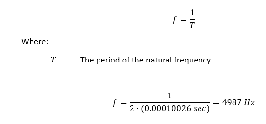
Let’s now visit the aspect of setting up a transient structural analysis, and specifically address the time-period associated with our event and determine how we can estimate this period for any geometry.
If we look at the time when the blue line crossed from negative displacement to positive displacement (0.00010026 seconds) which equals the period associated with the compression of our shaft.
Our shaft can be considered a spring that bounces. The duration of impact is reflective of ½ the period of its natural frequency in the direction of compression. Therefore, the following should be true.
Now let’s explore whether we can support this theory, as well as how we can estimate the natural frequency for this, and any geometry for which we hope to analyze in the future.
We can change the “compression only” support applied to the test model above, with a Y-Direction constraint on those same surfaces and solve directly for our longitudinal vibration frequency in ANSYS.
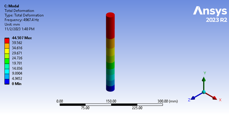
Figure 9: Modal Analysis Fundamental Frequency
Here we see the longitudinal vibration frequency is 4967.4 Hz. This shows that our estimation of natural frequency based on our transient structural displacement results was accurate to within 0.4%. This finding confirms our theory that the duration of impact equals ½ of the fundamental frequency’s period for the softer of two impacting objects.
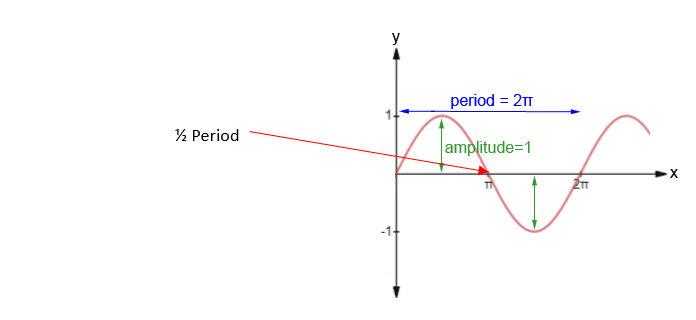
Figure 10: Impact Period
In our example analysis, we have only one part and we assume the compression only vertical support represents another very stiff object. Therefore, our shaft is the more flexible of these two impact partners. Our transient structural analysis was defined to have an analysis duration equal to the period of this natural frequency, and we expect impact to occur during the first ½ of this period.
But how do we calculate this natural frequency if we are setting up a transient structural analysis?
We can do as I just demonstrated, which is to perform a modal analysis of the geometry, while using constraints to maintain the impact posture and solve directly for the mode shape of impact compression. But is there an analytical way to accomplish the same thing?
To explore this, we need to calculate the natural frequency of our geometry in the direction of impact which can be calculated as follows.
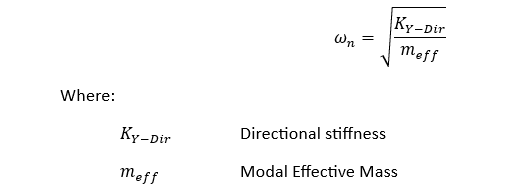
We already explored how we can estimate the directional stiffness, but now let’s consider a couple examples to better understand the consideration of modal effective mass.
The total mass of our system is:

The effective mass of our system will be less than the total mass, since one end of our geometry is constrained. It may be difficult to estimate the amount of mass that will participate based on the complexity of our geometry and the constraints used to fix the geometry. In our case, the geometry is simple and for extruded cross sections that are fixed on one end, the effective mass is often derived to equal 1/3 of the total mass of the system. If this were the case, then the following would be our fundamental frequency:

Which can be more recognizably be stated as:
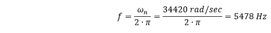
This value (5478 Hz) is over 10% larger than our natural frequency (4967.4 Hz) calculated by the finite element method… why?
The answer is related to the estimation of modal effective mass. If we feel confident in the calculation of longitudinal stiffness (…we do…), then we can change our model setup to more easily verify the calculation of our fundamental frequency.
We will set the mass density of our material for our model to equal zero, then add 1.01031 kg mass to the distal end of our geometry, which should produce the following natural frequency.
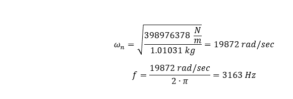
Having run the finite element analysis, we see the fundamental longitudinal frequency to be 3154.6 Hz.
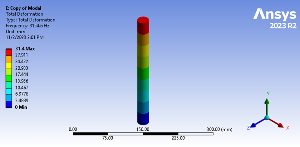
Figure 11: Modal Analysis Fundamental Frequency
This reflects a 0.27% difference from our hand calculation. Therefore, we develop more confidence in the finite element method, and identify a weakness in our estimation of the effective mass used in our hand calculation utilizing distributed mass throughout our geometry.
By re-arranging our equation, we can solve for this effective mass by considering the natural frequency calculated by ANSYS while considering distributed mass as follows:

We find this effective mass to be 0.405 of the total mass of the system.
Therefore, for other, and more complex geometries, we can expect this mass fraction to be unique and challenging to derive theoretically and that we can reliably solve for natural frequency using the finite element method.
Now that we understand how we will determine the natural frequency for a given geometry, we need to determine at what frequency we should collect analysis results during our transient analysis.
To do this, we should consider how the analysis step size impacts the analysis from two different perspectives. One perspective is in terms of what one could expect using a piecewise linear characterization of a non-linear response, such as a sine wave. The other perspective relates to how the actual analysis results change as a function of the change in the capture rate frequency. Because we are considering an impact problem and we have assumed that the impact period is associated with the fundamental vibration of our flexible component, it makes sense to explore the relationship between step size and how it impacts the accuracy representing a sinusoidal curve.
To evaluate this relationship, we will compare the weighted average of the magnitude for the first half of the sinusoidal curve to the theoretical average of this same span, which equals:

Now we explore how accurately, by using a different number of steps, we represent this sinusoidal curve, then use the trapezoidal rule to calculate the area under the curve for the first half, then divide that area by the period of that span.
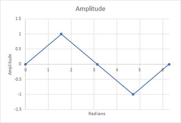
Figure 12: 4 Steps; Estimated Weighted Average=0.5; 21.46% Difference
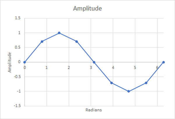
Figure 13: 8 Steps; Estimated Weighted Average=0.60536; 5.19% Difference
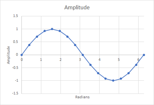
Figure 14: 16 Steps; Estimated Weighted Average=0.6284; 1.29% Difference
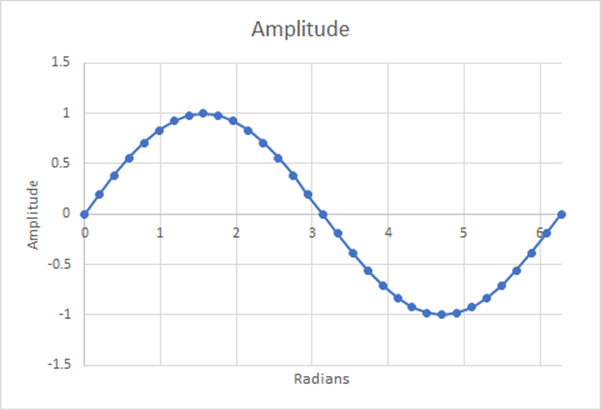
Figure 15: 32 Steps; Estimated Weighted Average=0.6346; 0.32% Difference
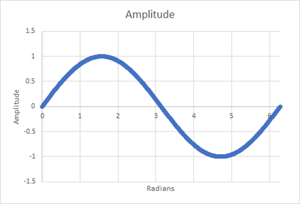
Figure 16: 512 Steps; Estimated Weighted Average=0.6366; 0.001% Difference
In fact, we never do achieve perfect agreement to the theoretical value, and we can plot how this accuracy changes as the number of time steps increases as illustrated below.
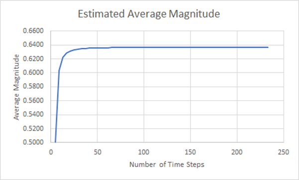
Figure 17: Estimated Average Magnitude Convergence Plot
From this examination, we can see that large increases in accuracy come quickly as we increase the number of steps in our approximation. But this does not consider how the results develop as the number of time steps are increased.
To explore the influence on analysis results, we will plot our maximum rod compression results, as a function of time, while considering different numbers of time-steps defined in the solution.
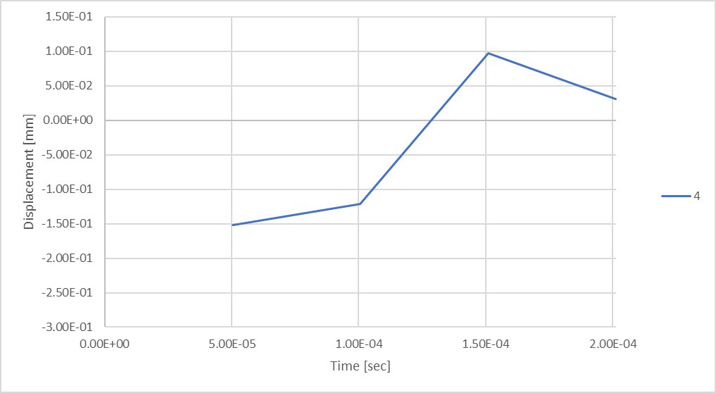
Figure 18: Rod Displacement while considering 4 time-steps.
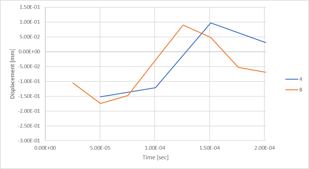
Figure 19: Rod Displacement while considering 8 time-steps.
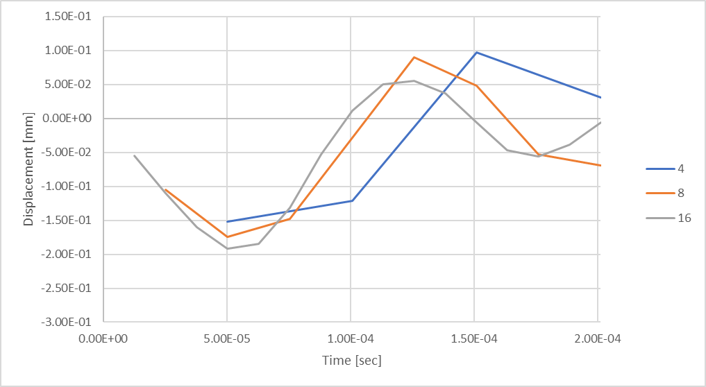
Figure 20: With 16 time-steps, we see larger rod compressive displacements.
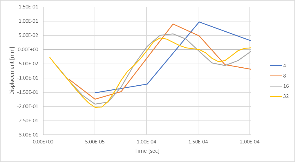
Figure 21: Transient Maximum Rod Deflection using 32 time-steps.
Based on our prior analysis of calculating average sinusoidal magnitude, we found that by considering 32 steps, we should expect up to 0.32% difference with theoretical results. But, we can see that our rod compressive displacement response is still being formed compared to the prior time-step explorations. What happens if we consider additional time-steps?
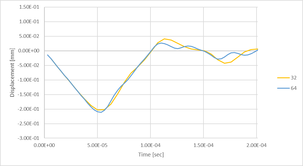
Figure 22: Transient Maximum Rod Deflection using 64 time-steps.
64 Time Steps produces slightly larger, but mostly similar maximum compressive rod deflection, however, there are signs of higher frequency oscillations being developed during the rebound of the rod.
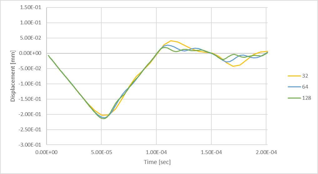
Figure 23: Transient Maximum Rod Deflection using 128 time-steps.
Considering 128 time-steps larger peak compression in the shaft over the lesser number of time-steps. The maximum compressive deflection is 6% larger than was produced while considering 32 time-steps.
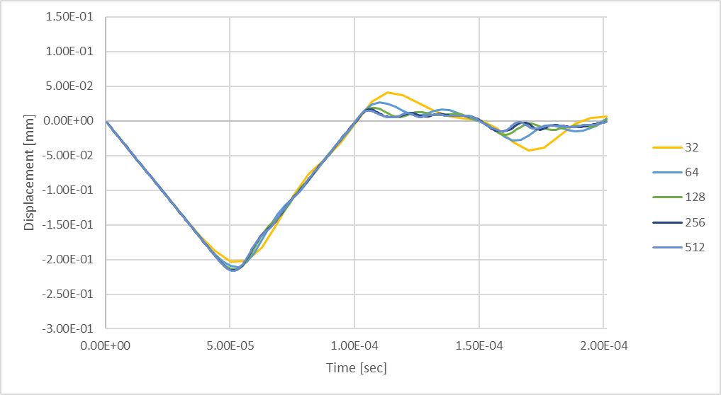
Figure 24: Transient Maximum Rod Deflection using up to 512 time-steps.
Comparing the 256 time-step analysis results with those produced by considering 512 time-steps shows that by considering more time-steps, further resolution of the dynamic response can be calculated. The following chart illustrates how one can expect our maximum compressive rod deflections will change as a function of the number of time-steps considered in a transient structural analysis.
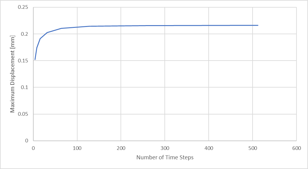
Figure 25: Maximum Rod Compressive Displacement vs Number of Analysis Time Steps
Eventually, for a given mesh size, we reach a point of diminishing returns… where the effort involved with extended analysis time and larger result files is not justified by significant change in results magnitude.
Based on these two considerations, we can see that by using 32 time-steps, we can expect to characterize a sinusoidal curve with up to 0.32% difference, but may only produce displacement results with 94% accuracy compared to the same analysis that utilized 512 time-steps, and only within 91% accuracy while compared to our theoretical maximum deflection. We see in the figure below how our maximum rod compression results compare to our theoretically estimated maximum.
| Number of Sub-Steps | Max Compression | Theoretical Max | % Difference |
| 4 | 0.152139 | 0.222859 | 31.73% |
| 8 | 0.174023 | 0.222859 | 21.91% |
| 16 | 0.191486 | 0.222859 | 14.08% |
| 32 | 0.202746 | 0.222859 | 9.03% |
| 64 | 0.210712 | 0.222859 | 5.45% |
| 128 | 0.214455 | 0.222859 | 3.77% |
| 256 | 0.215752 | 0.222859 | 3.19% |
| 512 | 0.216232 | 0.222859 | 2.97% |
Figure 26: Maximum Rod Compressive Displacement vs Analysis Time Steps
As the number of time-steps are increased, the agreement between our finite element analysis results and our theoretically derived value increases.
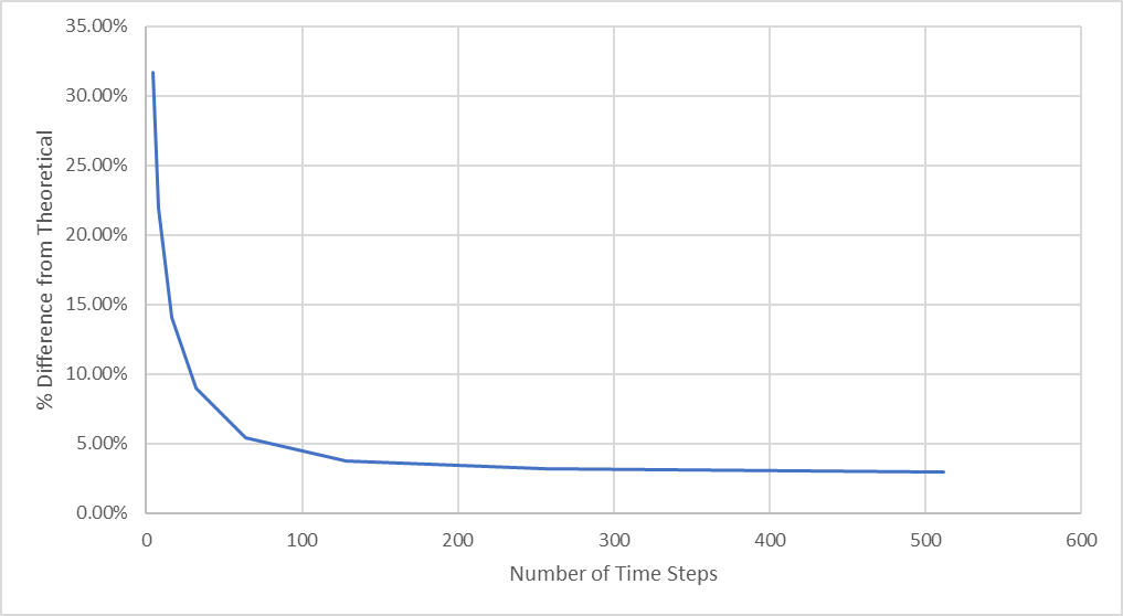
Figure 27: Percent Difference from Theoretical Maximum Deflection
We see from this figure how there is dramatic improvement towards convergence as the the number of time steps is between 64 and 128, but changes very little as the number of time steps are increased.
But what does all this mean in regard to other results, such as stress?
Below, I will plot the maximum von Mises stress per time for several analysis scenarios.
Figure 28: von Mises Stress while solving 32 time steps
Figure 29: von Mises Stress while solving 64 time steps
Figure 30: von Mises Stress while solving 128 time steps
Figure 31: von Mises Stress while solving 256 time steps
Figure 32: von Mises Stress while solving 512 time steps
In Summary, this is what we see while viewing stresses:
| Number of Sub-Steps | Max Average Stress | Maximum Peak Stress | % Difference of Average Stress |
| 4 | 120.04 | 301.98 | 29.62% |
| 8 | 136.4 | 316.61 | 20.03% |
| 16 | 150.57 | 312.42 | 11.72% |
| 32 | 159.15 | 301.68 | 6.69% |
| 64 | 165.4 | 283.51 | 3.03% |
| 128 | 168.84 | 303.99 | 1.01% |
| 256 | 170.05 | 354.35 | 0.30% |
| 512 | 170.56 | 442.08 | 0.00% |
Figure 33: Maximum Rod Compressive Displacement vs Analysis Time Steps
We can see that the peak impact stresses become larger as the number of time steps increase, showing the largest values at the onset of impact and becoming smaller throughout the event. The average stresses in the rod do ramp from zero to a peak at maximum compression, then fall back towards zero after impact has ended. We can plot these maximum average stresses below.
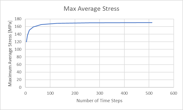
Figure 34: Maximum Rod Compressive Displacement vs Analysis Time Steps
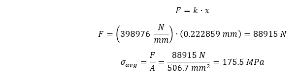
To put these maximum average stresses into perspective, we can calculate a theoretical maximum average stress in our rod as follows:
Plotting our maximum average stresses again vs our theoretically calculated maximum average allows us to summarize the % difference as follows:
| Number of Sub-Steps | Max Average Stress | Theoretical Maximum Average Stress | % Difference |
| 4 | 120.04 | 175.5 | 31.60% |
| 8 | 136.4 | 175.5 | 22.28% |
| 16 | 150.57 | 175.5 | 14.21% |
| 32 | 159.15 | 175.5 | 9.32% |
| 64 | 165.4 | 175.5 | 5.75% |
| 128 | 168.84 | 175.5 | 3.79% |
| 256 | 170.05 | 175.5 | 3.11% |
| 512 | 170.56 | 175.5 | 2.81% |
Figure 35: Maximum Rod Compressive Displacement vs Analysis Time Steps
Once again, just as was for the deflections, we acknowledge significant improvement in the percent difference of our maximum average stress compared to our theoretically calculated maximum average stress while considering between 64 and 128 time steps for the event. However, utilizing more time steps shows little improvement in the accuracy of our results.
Conclusion
We verify that the energy methods used to estimate maximum deflections and average stresses for the dynamic event, such as a drop of an elastic object on to a hard surface, may produce reasonable results and that the most significant improvements in accuracy occur while considering between 64 and 128 time steps for an event equal in period of the natural frequency of our impacting object, calculated for the direction of impact. We also found that the best method to approximate this natural frequency is not by hand calculations, but by a modal analysis performed using the finite element method, specifically because the amount of participating modal effective mass may not be easily estimated by any other method.
Please view Part 2 of this series, were we will consider our cylindrical rod as it impacts a more flexible plate, and apply what we have learned here in Part 1.
